Transcription
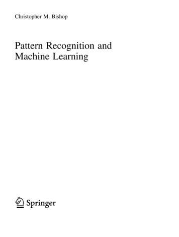
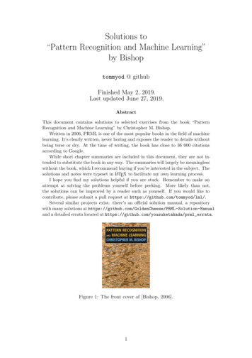
Solutions to“Pattern Recognition and Machine Learning”by Bishoptommyod @ githubFinished May 2, 2019.Last updated June 27, 2019.AbstractThis document contains solutions to selected exercises from the book “PatternRecognition and Machine Learning” by Christopher M. Bishop.Written in 2006, PRML is one of the most popular books in the field of machinelearning. It’s clearly written, never boring and exposes the reader to details withoutbeing terse or dry. At the time of writing, the book has close to 36 000 citationsaccording to Google.While short chapter summaries are included in this document, they are not intended to substitute the book in any way. The summaries will largely be meaninglesswithout the book, which I recommend buying if you’re interested in the subject. Thesolutions and notes were typeset in LATEX to facilitate my own learning process.I hope you find my solutions helpful if you are stuck. Remember to make anattempt at solving the problems yourself before peeking. More likely than not,the solutions can be improved by a reader such as yourself. If you would like tocontribute, please submit a pull request at https://github.com/tommyod/lml/.Several similar projects exist: there’s an official solution manual, a repositorywith many solutions at aland a detailed errata located at https://github.com/yousuketakada/prml errata.Figure 1: The front cover of [Bishop, 2006].1
Contents1 Chapter summaries1.1 Introduction . . . . . . . . . . .1.2 Probability Distributions . . . .1.3 Linear Models for Regression .1.4 Linear Models for Classification1.5 Neural networks . . . . . . . .1.6 Kernel methods . . . . . . . . .1.7 Sparse Kernel Machines . . . .1.8 Graphical Models . . . . . . . .1.9 Mixture Models and EM . . . .1.10 Approximate Inference . . . . .1.11 Sampling Methods . . . . . . .1.12 Continuous Latent Variables . .1.13 Sequential Data . . . . . . . . .1.14 Combining Models . . . . . . .336911121416182122242629302 Exercises2.1 Introduction . . . . . . . . . . .2.2 Probability Distributions . . . .2.3 Linear Models for Regression .2.4 Linear Models for Classification2.5 Neural networks . . . . . . . .2.6 Kernel methods . . . . . . . . .2.7 Sparse Kernel Machines . . . .2.8 Graphical Models . . . . . . . .2.9 Mixture Models and EM . . . .2.10 Approximate Inference . . . . .2.11 Sampling Methods . . . . . . .2.12 Continuous Latent Variables . .2.13 Sequential Data . . . . . . . . .31313644475259626471768283862
1Chapter summariesNotationScalar data is given by x (x1 , . . . , xN )T , where N is the number of samples. Vectordata is given by X, which has dimensions N M , where N is the number of data points(rows) and M is the dimensionality of the feature space (columns).MathematicsSome useful mathematics is summarized here, also see the book appendix. The gamma function Γ(x) satisfies Γ(x) (x 1)Γ(x 1), and is given byZ ux 1 e u du.Γ(x) 0It’s a “continuous factorial,” which is proved by integration by parts and induction. The Jensen inequality states that, for convex functions!XXfλj xj λj f (xj ),jwhere1.1Pjjλj 1 and λj 0 for every j.IntroductionProbabilityThe joint probability is given by p(x, y), which is short notation for p(X xi Y yj ). The sum rule isp(x) XZp(x, y) p(x, y) dy.y– Applying the sum rule as above is called “marginalizing out y.” The product rule isp(x, y) p(x y)p(y).– Computing p(x y) is called “conditioning on y.” Let w be parameters and D be data. Bayes theorem is given byp(w D) p(D w)p(w)p(D) posterior likelihood prior.evidence– Frequentist: data D generated from a fixed w.– Bayesian: data D fixed, find best w given this data.3
Frequentists generally quantify the properties of data driven quantities in light ofthe fixed model parameters, while Bayesians generally quantify the properties ofunknown model parameters in light of observed data. See [VanderPlas, 2014].Expectation and covarianceLet x be distributed with density p(x), then The expectation of a function f (x) defined over x with probability density p(x) isZXE[f ] f (xj )p(xj ) f (x)p(x) dxj The variance of f (x) is var[f ] E (f E[f ])2 E[f 2 ] E[f ]2 The covariance of x and y given bycov[x, y] Ex,y [(x E[x])(y E[y])] The covariance matrix Σ has entries σij corresponding to the covariance of variablesi and j. Thus Σ I means no covariance. (Note that real data may have nocovariance and still be dependent, i.e. have predictive power, xj f (xk ) where f isnon-linear. See “Anscombe’s quartet” on Wikipedia.)Polynomial fittingPMjLet y(x, w) j 1 wj x be a polynomial. We wish to fit this polynomial to valuesx (x1 , . . . , xN ) and t (t1 , . . . , tN ) i.e. a degree M polynomial fitting N data points. The maximum likelihood solution is to minimizeE(w, x) NX[y(xn , w) tn ]2 .n 1e Regularization adds a weight-dependent error so that E(w,x) E(w, x) E(w).For instance, Ridge minimizes the 2-norm:eE(w,x) NX[y(xn , w) tn ]2 λ kwk22n 1While LASSO (Least Absolute Shrinkage and Selection Operator) minimizes anderror with the 1-norm. Both are examples of Tikhonov regularization.4
GaussiansThe multivariate Gaussian is given byN (x µ, Σ) 1(2π)D/2 Σ 1/2 1T 1exp (x µ) Σ (x µ)2where µ is the mean and Σ is the covariance. Working with the precision Λ : Σ 1 issometimes easier.Parameter estimationLet x {x1 , . . . , xN } be a data set which is identically and independently distributed(i.i.d). The likelihood function for the Gaussian isp x µ, σ2 NY N xj µ, σ 2 .j 1Estimates for the parameters θ (µ, σ 2 ) can be obtained by maximizing the likelihood,which is equivalent to maximizing the log-likelihood ln p (x µ, σ 2 ). Maximizing the likelihood p(D w) is equivalent to minimizing E eT e in polynomial fitting. Maximizing the posterior p(w D) (MAP) is equivalent to minimizing regularizedsum of squares E eT e λwT w.Model selection Both model and model hyperparameters must be determined.– Minimize the error over the test set. Balance bias and variance. High bias canlead to underfitting, high variance can lead to overfitting. Split data into training, testing and validation. If data is scarce, using K-fold cross validation is an option.Decision theory Assign x to a region Rj RM corresponding to a class Cj , which might or mightnot be the true class. Minimizing misclassification is done by assigning x to the Cj which maximizes theposterior p(Cj x). This is equivalent to maximizing chance of begin correct. Loss function Lk,j may be used, the loss function assigns a penalty when the trueclass and the predicted class differ. Lk,j 6 Lj,k in general. Pick the Cj whichminimizes expected loss, i.e. pick the class Cj which minimizesXLk,j p(x, Cj ).k5
Three general decision approaches in decreasing order of complexity: (1) inference withclass conditional probabilities p(x Cj ), (2) inference with posterior class probabilitiesp(Cj x) and (3) discriminant function.inferencexp(Ck , x)decisionCkdiscriminant functionInformation theory h(x) ln p(x) measures the degree of surprise. The entropy is the expected surprised, defined asH[p] E[h] XZp(xj ) ln p(xj ) p(x) ln p(x) dxjand measures how many nats are needed to encode the optimal transmission ofvalues drawn from p(x).– Discrete entropy is maximized by the uniform distribution.– Continuous (or differential) entropy is maximized by the Gaussian. Conditional entropy is given byZZXH[x y] p(xi , yj ) ln p(xi yj ) p(x, y) ln p(xi yj ) dx dy,i,jand we have that H[x, y] H[y x] H[x]. The Kullback-Leibner divergence is given by Zq(x)KL(pkq) p(x) lndxp(x)and is interpreted as the additional information needed if using q(x) to encode valuesinstead of the correct p(x).1.2Probability DistributionsConjugate priors Since we know thatp(w D) p(D w) p(w)posterior likelihood priorwe seek probability density functions such that the left hand side and the right handside is of the same functional form. In other words, the likelihood p(D w) is fixed,6
and we seek priors p(w) such that posterior p(w D) is of the same functional form.The idea is similar to eigenfunctions. Example: Since the binomial distribution is proportional to pk (1 p)n k , the Betadistribution, proportional to pα 1 (1 p)β 1 , is a conjugate prior. The product ofthese distributions then ensures that the posterior is of the same functional form asthe prior.ParameterConjugate priorµ in GaussianGaussianp in BinomialBeta-distributionp in Multinomial Dirichlet-distributionThe multidimensional Gaussian Gaussians arise naturally in sums x1 · · · xN and averages, since when N the sum is normally distributed by the central limit theorem. The multidimensional Gaussian can be diagonalized by diagonalizing the precisionmatrix Λ Σ 1 , then exp(xT Λx) exp(y T Dy), where D diag(d1 , . . . , dD ). One limitation is the unimodal nature of the Gaussian, i.e. it has a single peak. Partitioned Gaussians. Let x N (x µ, Σ), where Λ Σ 1 and xaµaΣaa Σabx µ Σ .xbµbΣba Σbb .– Conditional distributionp(xa xb ) N (x µa b , Λ 1aa ) 1µa b µa Λaa Λab (xb µb )– Marginal distributionp(xa ) N (xa µa , Σaa )7
– These results are proved using inverse of 2 2 block matrices and examiningthe quadratic and linear terms in the exponential. There also exist closed-form expressions for Bayes theorem when the prior andlikelihood are Gaussians with linear relationship.Bayesian inference Gaussian variables.– To estimate µN (σ 2 is assumed known), use Gaussian prior.– To estimate λ 1/σ 2 , use Gamma function as prior, i.e.Gam(λ a, b) The–––ba λa 1exp( bλ)Γ(a)since it has the same functional form as the likelihood.Student-t distribution may be motivated by:Adding an infinite number of Gaussians with various precisions. It’s the distribution of the sample mean (X̄ µ)/(S/ n) when x1 , . . . , xN arei.d.d. from a Gaussian.As the degrees of freedom df , the Student-t distribution converges to aGaussian. An important property of the Student-t distribution is it’s robustnessto outliers.Periodic variables The mean can be measured as θ̄, where we think of the data as lying in a circle. The von-Mises distribution is a Gaussian on a periodic domain. It is given byp(x θ0 , m) 1exp [m cos(θ θ0 )] .2πI0 (m)The exponential family The exponential family is given by p(x η) g(η)h(x) exp η T u(x)and many probability functions are members of this family. The entries of the vectorη are called natural parameters, and g(η) is a normalization constant.P Maximum likelihood depends only on the sufficient statistics n u(xn ). Non-informative priors make few assumptions, letting the data speak for itself.8
Nonparametric methods The general equation for density estimation isp(x) 'KNVwhere K is the number of points in a neighborhood of volume V and N is the totalnumber of points. Kernel functions (or Parzen windows) estimate a neighborhood giving decreasingweight to samples further away, e.g. a Gaussian kernel. The volume V is fixed, thedata (and kernel function) determines K. Nearest neighborhood fixes K, letting V be a function of the data.1.3Linear Models for RegressionLinear basis function models We assume the dependent data y may be written asy(x, w) M 1Xwj φj (x) wT φ(x).j 0– The function y(x, w) is linear in w, but not necessarily in x since φj (·) mightbe a non-linear function. It’s called a linear model because it’s linear in w.– Choices for the functions {φj } include identity, powers of x, Gaussians, sigmoids, Fourier basis, Wavelet basis, and arbitrary non-linear functions. Assuming a noise term N (0, β 1 ), the maximum-likelihood solution is 1 TwML ΦT ΦΦ t Φ† t,where Φ† is the Moore-Penrose pseudoinverse and the design matrix Φ has entriesΦij φj (xi ). The ML solution is equivalent to minimizing the sum of squares. Sequential learning is possible with e.g. the gradient descent algorithm, which isused to compute w(τ 1) wτ η En . This facilitates on-line learning. If there are multiple outputs which are linear in the same set of basis functions, thesolution is wk Φ† tk for every output k, and the system decouples. Regularizing the error E(w) with a quadratic term αwT w/2 has ML solution αI ΦT Φ w ΦT t.The solution above is equivalent to a prior p(w α) N (w 0, α 1 I).9
The Bias-Variance decomposition The bias-variance decomposition isexpected loss (bais)2 variance noise. Imagine drawing many data sets D from a distribution p(t, x).– The bias is the distance from the average prediction to the conditional expectation f (x) E [t x]. In other words: Bias fˆ(x) E fˆ(x) f (x)– The variance is the variability of y(x; D) around it’s average. Var fˆ(x) E[fˆ(x)2 ] E[fˆ(x)]2 Flexible models have high variance, while rigid models have high bias.Bayesian linear regression We introduce a parameter distribution over w, for instance an isotropic Gaussiandistribution with covariance matrix S0 α 1 I.p(w) N (w m0 , S0 )Although the prior p(w) is isotropic, the posterior p(w t) need not be.p(w) N (w m0 , S0 )p(t w) NY(prior)p(tn w)(likelihood)n 1p(w t) N (w mN , SN )(posterior) Analytical calculations are possible, leading to refinement of the posterior distribution of the parameters w as more data is seen. A predictive distribution p(t t, α, β) can be found. The predictive distribution accounts for uncertainty of the parameters α and β. The model may be expressed via an equivalent kernel k(x, xn ) asy(x, w) y(x, mN ) βφ(x)SN ΦT t NXβφ(x)T SN φ(xn ) tn {z}n 1k(x,xn )In this context, a kernel is a “similarity function,” a dot product in some space.This can reduce to lower dimensions and make computations faster.10
Bayestian model selection and limitations Bayestian model selection uses Bayes theorem with models {Mi } and data D asp(Mi D) p(D Mi )p(Mi )p(D)where Mi is a model (distribution). It’s possible to choose the best model giventhe data by evaluating the model evidence (or marginal likelihood ) p(D Mi ) viamarginalization over w. Some disadvantages of the simple linear model includes the fact that the functionsφj (x) are fixed before data is observed, and the number of functions often growexponentially with the number of inputs. These shortcomings are often alleviatedin other models by the fact that data typically lies on a lower-dimensional manifold.1.4Linear Models for ClassificationLeast squares and Fisher’s linear discriminant The following are non-probabilistic models, where the output is not a probability. Least squares classification minimizes a quadratic error function, and is analyticallytractable. The results are not probabilities, the method is very sensitive to outliers,and does not necessarily give good results even when the data is linearly separable. Fisher’s linear discriminant seeks to find w to minimizeJ(w) between class variancew T SB w .Tw SW wwithin class varianceThe method projects data to a (hopefully) desirable subspace, where generative or 1discriminative methods may be used. Solved by w SW(m2 m1 ). The perceptron algorithm find a separating plane if the data is linearly separable,but does terminate otherwise. Historically important.Generalized linear models and probabilistic generative models A generalized linear model (GLM) is of the form y(x) f wT x w0 , where theactivation function f (·) may be non-linear. A probabilistic model first models p(x Ck ) and p(Ck ), and then uses Bayes theoremto model p(Ck x). From Bayes theorem, we havep(C1 x) 1p(x C1 )p(C1 ) ,p(x C1 )p(C1 ) p(x C2 )p(C2 )1 exp( a) {z}the sigmoid σ(a)where a ln (p(x C1 )p(C1 )) ln (p(x C2 )p(C2 )). If we assume normal distributionswith shared covariance matrices, then a(x) is linear in x.11
Probabilistic discriminative models A probabilistic model finds p(Ck x) directly, without modeling the class-conditionaldistribution of p(x Ck ). In other words, we can determine w in the GLM y(x)T2f w x w0 directly. This entails fitting O(M ) coefficients instead of O(M ). To find w in y(x) σ wT x w0 , we minimize the cross entropy, given by thenegative log-likelihoodMXtn ln(yn ) (1 tn ) ln(1 yn ) .E(w) ln p(t w) {z} {z }n 1cross entropylikelihood Using the Newton-Raphson methodwn 1 wn H 1 (wn ) E(wn )on the error function E(w) is an instance of the iterative reweighed least squares(IRLS) method. Every step involves a weighted least squares problem, and E(w)has a unique global minimum.The Laplace approximation The idea behind the Laplace approximation is to place a normal distribution on amode z0 of the function f (z) 1Tf (z) ' f (z0 ) exp (z z0 ) A(z z0 )A ln f (z) z z02 One application of Laplace approximation is Bayesian logistic regression, which isgenerally intractable. Using the Laplace approximation, an approximation to exactBayesian inference is possible.1.5Neural networksThe basic idea of neural networks A neural network has a fixed number of adaptable basis functions. Unlike thealgorithms considered so far, neural networks let the activation functions themselvesbe learned, not just the weights of their linear combinations. The notation is:(3)wki(2)(1)xi , i 1, . . . , Dwjizj , j 1, . . . , M12wkjyk , k 1, . . . , K
In a two-layer network, the equation for the output is X XMM(2)(1)yk σ,wkj hwji xij 0i 0 {zzj}where σ(·) and h(·) are the activation functions in the final (3rd) and hidden (2nd)layer, respectively. They may differ in general.– In regression problems, the final activation function σ(·) is often the identity,and the error E(w) is the sum-of-squares error.– In regression problems, the final activation function σ(·) is often the softmax,and the error E(w) is the cross entropy. To see how the first layer learns activation functions, consider a D-D-2 network withsoftmax activation functions trained using cross entropy error. The first part of thenetwork learns non-linear functions φj (x), which are used for logistic regression inthe second part. This is perhaps best seen if we write X XDD(2)(1)yk σwkj φj (x) ,φj (x) hwji xi .j 0i 0Network training Network training involves finding weights w to minimize E(w), this is a non-convexoptimization problem, typically solved iteratively, i.e.wk 1 wk wk where wk is some update rule. For instance wk η E wk for gradientdescent, which requires gradient information. Computing the gradient w E wk is done using back-propagation, which is application of the chain rule of calculus to the network. First information is propagatedforward in the network, then an error is computed and the wjk E are found bypropagating information backward in the network. Second order derivatives, i.e. the Hessian H E, may be approximated orcomputed. Approximation schemes include diagonal approximation, outer productapproximation, inverse from outer product (using the Woodbury matrix identity)and finite differences. Exact evaluation is also possible, and computing fast multiplication is possible by considering the operator R{·} in v T H v T E R{ E}.Neural network regularizatione Naively adding a regularization term such as E(w E(w) αwT w/2 will beinconsistent with scaling properties. A better regularization is to useα1 X 2 α2 X 2w w2 w W2 w W1213
where W1 denotes (non-bias) weights in layer 1.– The regularization above is called weight-decay, since it corresponds to decayingweights while training by multiplying with a factor between 0 and 1. It can beshown thatweight decay early stopping. Four ways to learn invariance is– Augmenting the training data while learning, using some function s(x, ξ),where s(x, 0) x. As an example, the function might rotate an image slightly.– Use tangent propagation regularization to penalize the Jacobian of theneural network, with no penalization along the tangent of the transformation.– Pre-process the data and extract invariant features by hand.– Build invariance into the structure of the neural net, e.g. CNNs.– It can be shown thataugmenting data while learning tangent propagation regularizer.Soft weight sharing and mixture density networks Using soft weight sharing, we assume a Gausian mixture distribution as a prior overthe weights in the network. Mixture density networks work well for inverse problems, where p(t x) might bemultimodal. The approach is to use a neural network to learn πk , µk and σk2 in themixture densityKX p(t x) πk N t µk (x), Iσk2 (x) .k 1The {πk } have softmax activations in the output to enforce the summation constraint, while the {σk2 (x)} have exponential activations to enforce positivity. A full Bayesian treatment of neural networks is not analytically intractable. However, using the Laplace approximation for the posterior parameter distribution, andalternative re-estimation of α and β it is possible to use approximate evidence approximation.1.6Kernel methodsIntroduction to kernel methods The dual representation expresses a prediction y(x) wT φ(x) entirely in termsof the N seen data points by use of the kernel k(x, x0 ) φ(x)T φ(x). This is incontrast to learning weights w. The dual formulation of Ride regression isy(x) k(x)T (K λI) 1 t,14(1)
where k(x)T (k(x1 , x), k(x2 , x), . . . , k(xN , x)) and Knm k(xn , xm ).– Typically the number of data points N is much greater than the dimensionalityM of the features φ(x). Since (1) needs to invert K RN N , it’s not obviouslyuseful. One advantage is that infinite dimensional feature mappings need notbe computed explicitly. A simple example is φ(x) (1, x, x2 , . . .), which isinfinite dimensional, but k(x, x0 ) becomes (1 x2 ) 1 .– A kernel is valid if it corresponds to an inner product a feature space. A kernelis valid if K is positive definite for every possible x. Valid kernels may beconstructed from other valid kernels, for instancek k1 k2 ,k k1 k2 ,k exp(k1 ),.This is called kernel engineering. Kernel regression (the Nadaraya-Watson model) models p(x, t) asN1 Xf (x xn , t tn ).p(x, t) N n 1Gaussian processes A prior over weights w p(w), implicitly defines a distribution over functionsy(x) wT φ(x). Predictions on a finite set of values is given by y Φw. Formulated in term of kernels, a Gaussian process is specified byE [y(xn )y(xm )] k(xn , xm ) cov [y] . The kernel may for instance be given by θ1k(xn , xm θ) φ0 exp kxn xm k θ2 θ3 xTn xm .2If xn xm , then the kernel will be comparatively large and the covariance will belarger. In other words; points that are close are more highly correlated. In Gaussian process regression, the predicted mean and variance is given byµ(XN 1 ) kT CN 1 tσ 2 (XN 1 ) c kT CN 1 k,where CN k(xn , xm ) β 1 δnm is the covariance matrix after observing N points.Hyperparameters and extensions Hyperparameters θ in k(xn , xm θ) can be optimized by maximizing the log likelihood ln p(t θ), which is in general non-convex. This is type 2 maximum likelihood. Gaussian processes can be used for classification, by composing the output with asigmoid so that y σ(a(x)). Not analytically tractable, but approximate methods exist: (1) variational inference, (2) expectation maximization and (3) Laplaceapproximation.15
1.5True functionPredicted meansSamples with noisePredicted 1.001.25Figure 2: Gaussian process regression on data from yi sin(xi ) .1.7Sparse Kernel MachinesSupport vector machinesFigure 3: Data which is linearly separable in the feature vector space φ(x), but not inx-space. The maximum margin hyperplane is non-linear in x-space. Source: Wikipedia. The main idea (when data is linearly separable) is to optimize w and b in the equation y(x) wT φ(x) b so that the separating hyperplane has a maximal margin.The points closest to the margin are called support vectors, and the hyperplanedepends only on these points. Lagrange multipliers and the Karush-Kuhn-Tucker (KKT) conditions are needed tosolve the problem. For the problem below, the Lagrangian is L(x, λ) f (x) λg(x).Optimization problemminimize f (x)subject to g(x) 016KKT-conditionsg(x) 0, λ 0λg(x) 0
The KKT conditions must be true at the optimum. They state that each constraintis either active or inactive, and generalize Lagrange multipliers to deal with inequality constraints. The linearly separable classification problem has Lagrange functionNX12L(w, b, a) kwk an (tn yn 1) .2n 1Differentiating with respect to w and b, and substituting back into the Lagrangefunction yields the dual form of the optimization problembL(a) NNXN1XXan am tn tm k(xn , xm )an 2 n 1 m 1n 1(2)which is expressed entirely in terms of theP kernel k(xn , xm ) and the lagrange multipliers. TheP constraints are an 0 and n an tn 0, and predictions are given byy(x) n an tn k(xn , x) b. Since an 0 when point n is not a support vector (theconstraint is inactive), prediction relies only on the support vectors. The linearly inseparable classification problem minimizesCNXξn n 11kwk2 ,2where ξn are slack variables and the constraint is tn yn 1 ξn instead of tn yn b1. The dual Lagrangian function L(a)is exactly equalP to Equation (2), but theconstraints are now 0 an C (box constraints) and n an tn 0. The optimization problems above are quadratic programs (QP), and specializedmethods for solving QP for SVMs exist: chunking, decomposition methods andsequential minimal optimization. The problems are often large, since k(xn , xm )must be evaluated for every pair of points. The regression problem introduces a more robust error function1Xλ(yn tn )2 kwk22 n2CXE (yn tn ) n1kwk2 ,2where E (·) increases linearly outside of a margin of width 2 . Two slack variablesξn 0 and ξbn 0 are introduced, and minimizing the above is equivalent tominimize Cbξ,ξ,wXn1(ξn ξbn ) kwk2 ,2b ab ) is again quadratic. The resulting optimization problem is a QP.and L(a, The ν-SVM is mathematically equivalent to the above, but uses a parameter ν whichcontrols the fraction of the data points that become support vectors. This is a moreintuitive parameterization.17
Relevance vector machines For regression, the model and prior are formulated asp(t x, w, β) N (t y(x, w), β 1 ),where y(x, w) Xwn k(xn , x) bnp(w α) MYN (wi 0, αi 1 ).iThe name relevance vector machine comes from the fact that automatic relevancedetermination is used to infer the important data points in an SVM-like functiony(x, w), and these relevance vectors are analogous to support vectors. The hyperparameters {αi } and β are efficiently determined through re-estimationequations. The expectation maximization algorithm is also an option. The model is typically very sparse, even more sparse than SVM, as many of the {αi }are driven to infinity. The downside is that the optimization problem is non-convex,and in general takes O(M 3 ) time, where M N 1 if a SVM-like kernel is used.For classification, Laplace approximation may be used to derive results.1.8Graphical ModelsxnαtnwNσ2btxbFigure 4: A graphical model for polynomial regression. Model parameters are shownwithout circles (e.g. σ 2 ), random variables are encircled (e.g. xn ), observed randomvariables are shaded (e.g. tn ) and plate notation is used to repeat the enclosed nodes.Directed graphs A graph is associated with a factorization of the joint probability density functionp(x). For instance, the graph below means that p(x) can be factored as p(x1 x2 )p(x2 )p(x3 x2 ). It imposes structure on p(x) by it’s lack of edges.x1x218x3
Approaches to reducing the number of model parameters include:– Removing edges: induces factorization properties on p(x).– Sharing parameters: merging parents together into a common node. – Restricting the functional form: for instance assuming p(y 1 x) σ wT x . The three examples below demonstrate conditional independence properties in simple directed graphs. Observing c blocks the tail-to-tail and head-to-tail paths, butobserving c (or any descendant of c) unblocks the head-to-head path.acabca 6 b acabca 6 b abca b cba b abca b cba 6 b c D-separation. Consider disjoint subsets A, B and C of edges in a graph. Let C beobserved. A path from A to B is said to be blocked if– There is a tail-to-tail or head-to-tail path with a node in C in the path.– There is a head-to-head path, where the middle not is not in C, nor any of it’sdescendants.If every path from A to B is blocked, then A B C. A graph can be thought of as a filter. The filter inputs are pdfs p(x), and thosefactoringQaccording to the given graph structure pass through the filter. For instance,p(x) i p(xi ) would pass any such filter. The set DF, for directed factorization,is the set of probability density functions passing through a specific filter. The Markov blanket of a graph is the minimal set of nodes that isolates xi from therest of the graph. In other words, p(xi x{i6 i} ) is only functionally dependent onthe nodes in the Markov blanket, which consists
\Pattern Recognition and Machine Learning" by Bishop tommyod @ github Finished May 2, 2019. Last updated June 27, 2019. Abstract This document contains solutions to selected exercises from the book \Pattern Recognition and Machine Learning" by Christopher M. Bishop. Written in 2006, PRML i


