Transcription
Modelling, Simulationand Control in MATLABHans-Petter Halvorsenhttps://www.halvorsen.blog
Modelling, Simulation andControl in MATLAB
University of South-Eastern NorwayMATLABModelling, Simulation & ControlHans-Petter Halvorsen, 2022.05.24http://www.halvorsen.blog
PrefaceCopyright You cannot distribute or copy this document withoutpermission from the author. You cannot copy or link to this documentdirectly from other sources, web pages, etc. You should always link to theproper web page where this document is located, typicallyhttp://www.halvorsen.blogIn this MATLAB Course, you will learn basic MATLAB and how to useMATLAB in Control and Simulation applications. An introduction toSimulink and other Tools will also be given.MATLAB is a tool for technical computing, computation and visualization inan integrated environment. MATLAB is an abbreviation for MATrixLABoratory, so it is well suited for matrix manipulation and problemsolving related to Linear Algebra, Modelling, Simulation and Controlapplications.This is a self-paced course based on this document and some short videoson the way. This document contains lots of examples and self-paced tasksthat the users will go through and solve on their own. The user may gothrough the tasks in this document in their own pace and the instructorwill be available for guidance throughout the course.The MATLAB Course consists of 3 parts:1. Introduction to MATLAB2. Modelling, Simulation and Control3. Simulink and Advanced TopicsIn Part 2 of the course you will learn how to use MATLAB in Modelling,Control and Simulation.You must go through MATLAB Course – Part 1: Introduction to MATLABbefore you start.The course consists of lots of Tasks you should solve while reading thiscourse manual and watching the videos referred to in the text.ii
Make sure to bring your headphones for the videos in thiscourse. The course consists of several short videos that will give you anintroduction to the different topics in the course.PrerequisitesYou should be familiar with undergraduate-level mathematics and haveexperience with basic computer operations.What is MATLAB? MATLAB is a tool for technical computing, computationand visualization in an integrated environment. MATLAB is an abbreviationfor MATrix LABoratory, so it is well suited for matrix manipulation andproblem solving related to Linear Algebra.MATLAB is developed by The MathWorks. MATLAB is a short-term forMATrix LABoratory. MATLAB is in use world-wide by researchers anduniversities. For more information, see www.mathworks.comFor more information about MATLAB, etc., please visithttp://www.halvorsen.blogOnline MATLAB ts/programming/matlab/MATLAB ming/matlab/matlab basics.phpModelling, Simulation and Control with ming/matlab/matlab mic.phpiii
MATLAB atlab basics videos.phpMATLAB for ing/courses/matlab.phpOn these web pages you find video solutions, complete step by stepsolutions, downloadable MATLAB code, additional resources, etc.iv
Table of ContentsPreface . iiTable of Contents . v1Introduction .12Differential Equations and ODE Solvers .22.1ODE Solvers in MATLAB .4Task 1: Bacteria Population.5Task 2: Passing Parameters to the model.6Task 3: ODE Solvers .72.1.1Higher order differential equations .8Task 4: 2. order differential equation . 143Discrete Systems . 163.1Discretization . 16Task 5: Discrete Simulation . 19Task 6: Discrete Simulation – Bacteria Population . 19Task 7: Simulation with 2 variables . 203.24Code Optimization . 20Numerical Techniques . 254.1Interpolation . 25Task 8: Interpolation . 274.2Curve Fitting . 284.2.1Linear Regression . 28Task 9: Linear Regression . 30v
viTable of Contents4.2.2Polynomial Regression . 31Task 10: Polynomial Regression . 33Task 11: Model fitting . 334.3Numerical Differentiation . 34Task 12: Numerical Differentiation . 384.3.1Differentiation on Polynomials. 39Task 13: Differentiation on Polynomials . 40Task 14: Differentiation on Polynomials . 404.4Numerical Integration . 40Task 15: Numerical Integration . 444.4.1Integration on Polynomials . 45Task 16: Integration on Polynomials . 455Optimization . 46Task 17: Optimization . 49Task 18: Optimization - Rosenbrock's Banana Function . 496Control System Toolbox . 517Transfer Functions . 537.1Introduction. 53Task 19: Transfer function . 557.2Second order Transfer Function . 56Task 20: 2.order Transfer function . 56Task 21: Time Response. 577.3Analysis of Standard Functions . 58Task 22: Integrator . 58Task 23: 1. order system. 58Task 24: 2. order system. 58MATLAB Course - Part II: Modelling, Simulation and Control
viiTable of ContentsTask 25: 2. order system – Special Case . 608State-space Models . 618.1Introduction. 618.2Tasks . 63Task 26: State-space model . 63Task 27: Mass-spring-damper system . 63Task 28: Block Diagram . 648.3Discrete State-space Models . 65Task 29: Discretization . 669Frequency Response. 679.1Introduction. 679.2Tasks . 70Task 30: 1. order system. 70Task 31: Bode Diagram . 719.3Frequency response Analysis. 729.3.1Loop Transfer Function . 729.3.2Tracking Transfer Function . 729.3.3Sensitivity Transfer Function . 73Task 32: Frequency Response Analysis . 749.4Stability Analysis of Feedback Systems . 75Task 33: Stability Analysis . 7710Additional Tasks . 78Task 34: ODE Solvers . 78Task 35: Mass-spring-damper system . 78Task 36: Numerical Integration . 79Task 37: State-space model . 80MATLAB Course - Part II: Modelling, Simulation and Control
viiiTable of ContentsTask 38: lsim . 80Appendix A – MATLAB Functions . 83Numerical Techniques . 83Solving Ordinary Differential Equations . 83Interpolation . 83Curve Fitting . 83Numerical Differentiation . 84Numerical Integration . 84Optimization . 84Control and Simulation . 85MATLAB Course - Part II: Modelling, Simulation and Control
1 IntroductionAdditional Resources, Videos, etc. are available ng/matlabPart 2: “Modelling, Simulation and Control” consists of the followingtopics: Differential Equations and ODE SolversDiscrete SystemsNumerical Techniqueso Interpolationo Curve Fittingo Numerical Differentiationo Numerical IntegrationOptimizationControl System ToolboxTransfer functionsState-space modelsFrequency Response1
2 Differential Equationsand ODE SolversMATLAB have lots of built-in functionality for solving differential equations.MATLAB includes functions that solve ordinary differential equations (ODE)of the form:𝑑𝑦 𝑓(𝑡, 𝑦),𝑑𝑡𝑦(𝑡! ) 𝑦!MATLAB can solve these equations numerically.Higher order differential equations must be reformulated into a system offirst order differential equations.Note! Different notation is used:𝑑𝑦 𝑦 " 𝑦̇𝑑𝑡This document will use these different notations interchangeably.Not all differential equations can be solved by the same technique, soMATLAB offers lots of different ODE solvers for solving differentialequations, such as ode45, ode23, ode113, etc.Example:Given the following differential equation:𝑥̇ 𝑎𝑥#where 𝑎 ,where 𝑇 is the time constantNote! 𝑥̇ %&%'The solution for the differential equation is found to be:𝑥(𝑡) 𝑒 (' 𝑥!We shall plot the solution for this differential equation using MATLAB.2
3SolversDifferential Equations and ODESet 𝑇 5 and the initial condition 𝑥(0) 1.We will create a script in MATLAB (.m file) where we plot the solution 𝑥(𝑡)in the time interval 0 𝑡 25The Code is as follows:T 5;a -1/T;x0 1;t [0:1:25]x exp(a*t)*x0;plot(t,x);gridThis gives the following Results:[End of Example]This works fine, but the problem is that we first have to find the solutionto the differential equation – instead we can use one of the built-in solversfor Ordinary Differential Equations (ODE) in MATLAB. In the examples andtasks below we will learn how we can use these built-in ODE solvers.There are different functions, such as ode23 and ode45.MATLAB Course - Part II: Modelling, Simulation and Control
4Solvers2.1Differential Equations and ODEODE Solvers in MATLABAll of the ODE solver functions (ode23, ode45, etc.) share a syntax thatmakes it easy to try any of the different numerical methods, if it is notapparent which is the most appropriate. To apply a different method tothe same problem, simply change the ODE solver function name. Thesimplest syntax, common to all the solver functions, is:[t,y] solver(odefun,tspan,y0,options, )where “solver” is one of the ODE solver functions (ode23, ode45, etc.).Note! If you don’t specify the resulting array [t, y], the function create aplot of the result.‘odefun’ is the function handler, which is a “nickname” for your functionthat contains the differential equations.Example:Given the following differential equation:𝑥̇ 𝑎𝑥#where 𝑎 ,where 𝑇 is the time constantWe use 𝑇 5 and the initial condition 𝑥(0) 1.We use the ode23 solver in MATLAB for solving the differential equation(“runmydiff.m”):tspan [0 25];x0 1;[t,x] ode23(@mydiff,tspan,x0);plot(t,x)Where @mydiff is defined as a function like this (“mydiff.m”):function dx mydiff(t,x)a -1/5;dx a*x;Note! You have to implement it in 2 different m. files, one m. file whereyou define the differential equation you are solving, and another .m filewhere you solve the equation using the ode23 solver.MATLAB Course - Part II: Modelling, Simulation and Control
5SolversDifferential Equations and ODEThis gives the same results as shown in the previous example above andMATLAB have solved the differential equation for us (numerically).[End of Example]Task 1: Bacteria PopulationIn this task we will simulate a simple model of a bacteria population in ajar.The model is as follows:birth rate bxdeath rate px2Then the total rate of change of bacteria population is:𝑥̇ 𝑏𝑥 𝑝𝑥 )Set b 1/hour and p 0.5 bacteria-hourNote! 𝑥̇ %&%' Simulate (i.e., create a plot) the number of bacteria in the jar after 1hour, assuming that initially there are 100 bacteria present.How many bacteria are present after 1 hour?[End of Task]MATLAB Course - Part II: Modelling, Simulation and Control
6SolversDifferential Equations and ODE2.1.1 Passing Arguments to the functionIn a differential equation we have different parameters that we may wantto change.Task 2: Passing Parameters to the modelGiven the following system:𝑥̇ 𝑎𝑥 𝑏#where 𝑎 ,where 𝑇 is the time constantIn this case we want to pass 𝑎 and 𝑏 as parameters, to make it easy tobe able to change values for these parameters.We set initial condition 𝑥(0) 1 and 𝑇 5. We can set 𝑏 1.The function for the differential equation is:function dx mysimplediff(t,x,param)% My Simple Differential Equationa param(1);b param(2);dx a*x b;Then we solve and plot the equation using this code:tspan [0 25];x0 1;a -1/5;b 1;param [a b];[t,y] ode45(@mysimplediff, tspan, x0,[], param);plot(t,y)By doing this, it is very easy to changes values for the parameters 𝑎 and𝑏 without changing the code for the differential equation.Note! We need to use the 5. argument in the ODE solver function for this.The 4. argument is for special options and is normally set to “[]”, i.e., nooptions.MATLAB Course - Part II: Modelling, Simulation and Control
7SolversDifferential Equations and ODEThe result from the simulation is: Write the code aboveTry also this techniqueon the following differential equation:𝑥̇ 𝑏𝑥 𝑝𝑥 )Set b 1/hour and p 0.5 bacteria-hourYou should also read more about the different solvers (ode34, ode 45,etc.) that exists in the Help system in MATLAB[End of Task]Task 3: ODE SolversUse the ode23 function to solve and plot the results of the followingdifferential equation in the interval [𝑡! , 𝑡* ]:𝒘" (𝟏. 𝟐 𝒔𝒊𝒏𝟏𝟎𝒕)𝒘 𝟎, 𝑡! 0, 𝑡* 5, 𝑤(𝑡! ) 1Note! 𝑤 " % %'[End of Task]MATLAB Course - Part II: Modelling, Simulation and Control
8SolversDifferential Equations and ODE2.1.2 Multiple 1. order DifferentialEquationsIn real life we typically have higher order differential equations, or wehave a set of 1. order differential equations that describe a given system.How can we solve such equations in MATLAB?Example:Given the differential equations:𝑑𝑦 𝑥𝑑𝑡𝑑𝑥 𝑦𝑑𝑡In MATLAB you define a function for these differential equations:function dy mydiff(t,y)dy(1) y(2);dy(2) -y(1);dy [dy(1); dy(2)];Note! Since numbers of equations is more than one, we need to usevectors!!Using the ode45 function gives the following code:[t,y] ode45(@mydiff, [-1,1], [1,1]);plot(t,y)title('solution of dy/dt x and dx/dt -y')legend('y', 'x')The equations are solved in the time span [ 1, 1] with initial values [1, 1].This gives the following plot:MATLAB Course - Part II: Modelling, Simulation and Control
9SolversDifferential Equations and ODENote! To make it more clearly, we can rewrite the equations (setting 𝑥# 𝑥, 𝑥) 𝑦):𝑑𝑥# 𝑥)𝑑𝑡𝑑𝑥) 𝑥#𝑑𝑡𝑥#𝑥̇Where we have the vector 𝑥 N𝑥 O and 𝑥̇ P # Q𝑥̇ ))or MATLAB “syntax”: 𝑑𝑥𝑑𝑡 𝑥̇In MATLAB it is tempting to define these 2 differential equations like this:dxdt1 -x2;dxdt2 x1;But if we have more than one differential equation (in this case wehave 2), we need to use vectors!So, it needs be like this:dxdt(1) -x(2);dxdt(2) x(1);The final code that implements the differential equations becomes(“mydiff.m”):MATLAB Course - Part II: Modelling, Simulation and Control
10SolversDifferential Equations and ODEfunction dxdt mydiff(t,x)dxdt(1) -x(2);dxdt(2) x(1);dxdt dxdt';Note! The function mydiff must return a column vector, that’s why weneed to transpose it.Then we use the ode solver to solve the differential equations(“run mydiff.m”):tspan [-1,1];x0 [1,1];[t,x] ode45(@mydiff, tspan, x0);plot (t,x)legend('x1', 'x2')The solution will be the same.[End of Example]2.1.3 Higher order differential equationsHigher order differential equations must be reformulated into a system offirst order differential equations.Example:Given the following "Mass-spring-damper" system:MATLAB Course - Part II: Modelling, Simulation and Control
11SolversDifferential Equations and ODEWhere t is the simulation time, F(t) is an external force applied to thesystem, c is the damping constant of the spring, k is the stiffness of thespring, m is a mass, and x(t) is the position of the mass.The goal is to view the position x(t) of the mass m with respect to time t.You can calculate the position by integrating the velocity of the mass. Youcan calculate the velocity by integrating the acceleration of the mass. Ifyou know the force and mass, you can calculate this acceleration by usingNewton's Second Law of Motion, given by the following equation:Force Mass AccelerationTherefore,Acceleration Force / MassWe can describe the system using a 2. order differential equation:𝐹(𝑡) 𝑐𝑥̇ (𝑡) 𝑘𝑥(𝑡) 𝑚𝑥̈ (𝑡)Where 𝑥̇ is the first derivative of the position, which equals the velocity ofthe mass. 𝑥̈ is the second derivative of the position, which equals theacceleration of the mass.We reformulate the differential equation so 𝑥̈ is alone on the left side.𝑥̈ 𝑘𝑐1𝑥 𝑥̇ 𝐹𝑚𝑚𝑚Higher order differential equations must be reformulated into a system offirst order differential equations.We set:𝑥# 𝑥𝑥) 𝑥̇ 𝑥̇ #This gives:𝑥̇# 𝑥)𝑥̇ ) 𝑥̈Finally:MATLAB Course - Part II: Modelling, Simulation and Control
12SolversDifferential Equations and ODE𝑥̇# 𝑥)𝑥̇ ) 𝑘𝑐1𝑥# 𝑥) 𝐹𝑚𝑚𝑚Now we are ready to solve the system using MATLAB.Below we present the MATLAB code.First, we need to create a function for our differential equations(mass spring damper diff.m):function dx mass spring damper diff(t,x)kmcF 1;5;1;1;dx zeros(2,1); %Initializationdx(1) x(2);dx(2) -(k/m)*x(1)-(c/m)*x(2) (1/m)*F;Then, we can write a MATLAB script (simulate mass spring damper.m)that is using this function as part of the built-in ode solver:clearclctspan [0 50];x0 [0;0];[t,x] ode23(@mass spring damper diff,tspan,x0);plot(t,x)This gives the following plot:MATLAB Course - Part II: Modelling, Simulation and Control
13SolversDifferential Equations and ODEIn the plot we see both 𝑥# and 𝑥) . If we only want to plot 𝑥# , we can dolike this:plot(t,x(:,2))Improved solution:For greater flexibility we want to be able to change the parameters k, m,c, and F without changing the function, only changing the script. A betterapproach would be to pass these parameters to the function instead.The updated function becomes:function dx mass spring damper diff2(t,x, param)kmcF param(1);param(2);param(3);param(4);dx zeros(2,1);dx(1) x(2);dx(2) -(k/m)*x(1) - (c/m)*x(2) (1/m)*F;The updated script becomes:clearMATLAB Course - Part II: Modelling, Simulation and Control
14SolversDifferential Equations and ODEclcclose alltspan [0 50];x0 [0;0];k 1;m 5;c 1;F 1;param [k, m, c, F];[t,x] ode23(@mass spring damper diff2,tspan,x0, [], param);plot(t,x)Then we can easily change the values k, m, c, and F.[End of Example]Task 4: 2. order differential equationUse the ode23/ode45 function to solve and plot the results of the followingdifferential equation in the interval [𝑡! , 𝑡* ]:(𝟏 𝒕𝟐 )𝒘̈ 𝟐𝒕𝒘̇ 𝟑𝒘 𝟐, 𝑡! 0, 𝑡* 5, 𝑤(𝑡! ) 0, 𝑤̇(𝑡! ) 1Note! 𝑤̈ %! %' !Note! Higher order differential equations must be reformulated into asystem of first order differential equations.Tip 1: Reformulate the differential equation so 𝑤̈ is alone on the left side.Tip 2: Set:𝑤 𝑥#𝑤̇ 𝑥)[End of Task]Example:Given the following differential equations:MATLAB Course - Part II: Modelling, Simulation and Control
15SolversDifferential Equations and ODE𝑥̇ # 0.9𝑥# 0.1𝑥) 1𝑥̇ ) 0.4𝑥) 0.8𝑥- 0.9𝑥̇ - 0.7𝑥# 0.1𝑥MATLAB:function dxdt my3orderdiff(t,x)dxdt(1) -0.9*x(1) 0.1*x(2) 1;dxdt(2) -0.4*x(2) 0.8*x(3) - 0.9;dxdt(3) -0.7*x(1) - 0.1*x(3);dxdt dxdt';and the Script for running the simulation:clearclctspan [0,30];x0 [0,0,0];[t,x] ode23(@my3orderdiff, tspan, x0);plot (t,x)legend('x1', 'x2', 'x3')[End of Example]MATLAB Course - Part II: Modelling, Simulation and Control
3 Discrete SystemsMATLAB has built-in powerful features for simulation of continuousdifferential equations and dynamic systems.Sometimes we want to or need to discretize a continuous system and thensimulate it in MATLAB.When dealing with computer simulation, we need to create a discreteversion of our system. This means we need to make a discrete version ofour continuous differential equations. Actually, the built-in ODE solvers inMATLAB use different discretization methods. Interpolation, Curve Fitting,etc. is also based on a set of discrete values (data points ormeasurements). The same with Numerical Differentiation and NumericalIntegration, etc.Below we see a continuous signal vs the discrete signal for a given systemwith discrete time interval 𝑇. 0.1𝑠.3.1DiscretizationIn order to discretize a continuous model there are lots of differentmethods to use. One of the simplest is Euler Forward method:𝑥̇ 𝑥/0# 𝑥/𝑇.16
17Discrete Systemswhere 𝑇. is the sampling time.Lots of other discretization methods do exists, such as “Euler backward”,Zero Order Hold (ZOH), Tustin’s method, etc.As shown in a previous chapter, MATLAB have lots of built-in functions forsolving differential equations numerically, but here we will create our owndiscrete model.Example:Given the following differential equation:𝑥̇ 𝑎𝑥 𝑏𝑢Note!𝑥̇ is the same as%&%'Where:𝑥 - Process variable, e.g., Level, Pressure, Temperature, etc.𝑢 - Input variable, e.g., Control Signal from the Controller𝑎, 𝑏 - ConstantsWe start with finding the discrete differential equation.We can use e.g., the Euler Approximation:MATLAB Course - Part II: Modelling, Simulation and Control
18Discrete Systems𝑥̇ 𝑥/0# 𝑥/𝑇.𝑇. - Sampling IntervalThen we get:𝑥/0# 𝑥/ 𝑎𝑥/ 𝑏𝑢/𝑇.This gives the following discrete differential equation:𝑥/0# (1 𝑇. 𝑎)𝑥/ 𝑇. 𝑏𝑢/Now we are ready to simulate the systemWe set 𝑎 0.25, 𝑏 2 and 𝑢 1 (You can explore with other values onyour own)The Code can be written as follows:% Simulation of discrete modelclear, clc% Model Parametersa 0.25;b 2;% Simulation ParametersTs 0.1; %sTstop 30; %suk 1; % Step Responsex(1) 0;% Simulationfor k 1:(Tstop/Ts)x(k 1) (1-a*Ts).*x(k) Ts*b*uk;end% Plot the Simulation Resultsk 0:Ts:Tstop;plot(k,x)grid onThis gives the following Results:MATLAB Course - Part II: Modelling, Simulation and Control
19Discrete Systems[End of Example]Task 5: Discrete SimulationGiven the following differential equation:𝑥̇ 𝑎𝑥#where 𝑎 , where 𝑇 is the time constantNote! 𝑥̇ %&%'Find the discrete differential equation and plot the solution for this systemusing MATLAB.Set 𝑇 5 and the initial condition 𝑥(0) 1.Create a script in MATLAB (.m file) where we plot the solution 𝑥(𝑘).[End of Task]Task 6: Discrete Simulation – Bacteria PopulationIn this task we will simulate a simple model of a bacteria population in ajar.MATLAB Course - Part II: Modelling, Simulation and Control
20Discrete SystemsThe model is as follows:birth rate bxdeath rate px2Then the total rate of change of bacteria population is:𝑥̇ 𝑏𝑥 𝑝𝑥 )Set b 1/hour and p 0.5 bacteria-hourWe will simulate the number of bacteria in the jar after 1 hour, assumingthat initially there are 100 bacteria present. Find the discrete model using the Euler Forward method by hand andimplement and simulate the system in MATLAB using a For Loop.[End of Task]Task 7: Simulation with 2 variablesGiven the following system𝑑𝑥# 𝑥)𝑑𝑡𝑑𝑥) 𝑥#𝑑𝑡Find the discrete system and simulate the discrete system in MATLAB.Solve the equations, e.g., in the time span [ 1 1] with initial values [1, 1].[End of Task]3.2Code OptimizationExample:When doing more advanced simulations, it is important that you spendtime optimization your code. In the examples and tasks above theequations are quite simple, but when the equations become moreMATLAB Course - Part II: Modelling, Simulation and Control
21Discrete Systemscomplicated, or your simulation time increases, code optimizationbecomes more important.In the code example below the following simple differential equation willbe used:𝑥̇ 𝑎𝑥 𝑏𝑢But we will increase the simulation time dramatically compared to theprevious examples.MATLAB Code 1;clear, clctica -10; b 0.5;x 0; u 1;dt 0.01;N 1000000000;X(1) x;for i 1:NX(i 1) X(i) dt*(a*X(i) b*u);endtocMATLAB Code 2:clear, clctica -10; b 0.5;x 0; u 1;dt 0.01;N 1000000000;X zeros(N,1);for i 1:NX(i 1) X(i) dt*(a*X(i) b*u);endtocMATLAB Code 3:clear, clctica -10; b 0.5;MATLAB Course - Part II: Modelling, Simulation and Control
22Discrete Systemsx 0; u 1;dt 0.01;N 1000000000;X zeros(N,1);for i 1:NX(i) x;x x dt*(a*x b*u);endtocTry the different code examples and note the execution time. Try withdifferent values of N, etc.[End of Example]Example:In the code example below the following simple differential equation willbe used:𝑥̇ 𝑎𝑥 𝑏𝑢MATLAB Code 1;% Simulation of discrete modelclear, clc% Model Parametersa 0.25;b 2;% Simulation ParametersTs 0.01;Tstop 10000000;x(1) 0;N Tstop/Ts;u linspace(0,1,N);% Simulationticfor k 1:Nx(k 1) (1-a*Ts).*x(k) Ts*b*u(k);endtoc% Plot the Simulation Resultst 0:Ts:Tstop;plot(t,x)grid onMATLAB Course - Part II: Modelling, Simulation and Control
23Discrete SystemsMATLAB Code 2:% Simulation of discrete modelclear, clc% Model Parametersa 0.25;b 2;% Simulation ParametersTs 0.01;Tstop 10000000;uk 1;N Tstop/Ts;u linspace(0,1,N);%Preallocationx zeros(N,1);% Simulationticfor k 1:Nx(k 1) (1-a*Ts).*x(k) Ts*b*u(k);endtoc% Plot the Simulation Resultst 0:Ts:Tstop;plot(t,x)grid onMATLAB Code 3:% Simulation of discrete modelclear, clc% Model Parametersa 0.25;b 2;% Simulation ParametersTs 0.01;Tstop 10000000;uk 1;x 0;X(1) x;N Tstop/Ts;u rand(N,1);u linespace(0,1,N);% SimulationX zeros(N,1);ticfor k 1:NMATLAB Course - Part II: Modelling, Simulation and Control
24Discrete Systemsx (1-a*Ts)*x Ts*b*u(k);X(k 1) x;endtoc% Plot the Simulation Resultst 0:Ts:Tstop;plot(t,X)grid onIn general, it will be many ways to implement a given system in MATLAB,we can use built in ODE solvers, we can use different discretizationmethods, and we can optimize our code in other ways.There is not a “best way” that can be used for all kind of systems. It willbe your responsibility to find the best solution for your system. That’s whyit is important that you know about different ways to do things, so you areable to find the best solution in a given situation.[End of Example]MATLAB Course - Part II: Modelling, Simulation and Control
4 Numerical TechniquesIn the previous chapter we investigated how to solve differential equationsnumerically, in this chapter we will take a closer look at some othernumerical techniques offered by MATLAB, such as interpolation, curvefitting, numerical differentiations and integrations.4.1InterpolationInterpolation is used to estimate data points between two known points.The most common interpolation technique is Linear Interpolation.In MATLAB we can use the interp1 function.Example:Given the following data:x012345y15109620We will find the interpolated value for 𝑥 3.5.The following MATLAB code will do this:x 0:5;y [15, 10, 9, 6, 2, 0];plot(x,y ,'-o')% Fin
MATLAB have lots of built-in functionality for solving differential equations. MATLAB includes functions that solve ordinary differential equations (ODE) of the form: ( , ), ( 0) 0 MATLAB can solve these equations n