Transcription
Linear Algebra and Differential EquationsAlexander GiventalUniversity of California, Berkeley
ContentForeword1. Geometry on the plane.1.1. Vectors1.1.1.Definitions. 1.1.2. Inner product. 1.1.3. Coordinates.1.2. Analytical geometry.1.2.1. Linear functions and staright lines. 1.2.2. Conic sections.1.2.3. Quadratic forms.1.3. Linear transformations and matrices.1.3.1. Linearity. 1.3.2. Composition. 1.3.3. Inverses. 1.3.4. Matrix Zoo.1.4. Complex numbers.1.4.1. Definitions and geometrical interpretations. 1.4.2. The exponential function.1.4.3. The Fundamental Theorem of Algebra.1.5. Eigenvalues.1.5.1. Linear systems. 1.5.2. Determinants. 1.5.3. Normal forms.Sample midterm exam2. Differential equations.2.1. ODE.2.1.1. Existence and uniqueness of solutions. 2.1.2. Linear ODE systems.2.2. Stability.2.2.1. Partial derivatives. 2.2.2. Linearization. 2.2.3. Competing species.2.3. PDE.2.3.1. The heat equation. 2.3.2. Boundary value problems.2.4. Fourier series.2.4.1. Fourier coefficients. 2.4.2. Convergence. 2.4.3. Real even and odd functions.2.5. The Fourier method.2.5.1. The series solution. 2.5.2. Properties of solutions.Sample midterm exam3. Linear Algebra.3.1. Classical problems of linear algebra3.2. Matrices and determinants.3.2.1. Matrix algebra. 3.2.2. The determinant function.3.2.3. Properties of determinants. 3.2.4. Cofactors.3.3. Vectors and linear systems.3.3.1. 3D and beyond. 3.3.2. Linear (in)dependence and bases.3.3.3. Subspaces and dimension. 3.3.4. The rank theorem and applications.3.4. Gaussian elimination.3.4.1. Row reduction. 3.4.2. Applications.v
viCONTENT3.5. Quadratic forms.3.5.1. Inertia indices. 3.5.2. Least square fitting to data. 3.5.3. Orthonormal bases.3.5.4. Orthogonal diagonalization. 3.5.5. Small oscillations.3.6. Eigenvectors.3.6.1. Diagonalization theorem. 3.6.2. Linear ODE systems.3.6.3. Higher order linear ODEs.3.7. Vector spaces.3.7.1. Axioms and examples. 3.7.2. Error-correcting codes.3.7.3. Linear operators and ODEs. 3.7.4. The heat equation revisited.Sample final exam.
ForewordTo the student:The present text consists of 130 pages of lecture notes, including numerouspictures and exercises, for a one-semester course in Linear Algebra and DifferentialEquations. The notes are reasonably self-contained. In particular, prior knowledgeof Multivariable Calculus is not required. Calculators are of little use. Intelligent,hands-on reading is expected instead.A typical page of the text contains several definitions. Wherever you see a wordtypeset in the font Sans Serif, it is a new term and the sentence is the definition.A large portion of the text represents Examples. However, numerical illustrations or sample solutions to homework problems are rare among them. Theexamples are there because they are part of the theory, and familiarity with eachone of them is crucial for understanding the material. Should you feel the need tosee numbers instead of letters, you are welcome to substitute your favorite ones.The notes are written in a concise, economical style, so do not be misled bythe total size of the text: you can find there more material than you can think of.If you notice that reading a typical page takes less than an hour, it is a clear signthat your reading skills may need further polishing. Ask your instructor to giveyou some hints. Perhaps they will sound like this:“Have you found out how the first sentence in a section implies the next one,the third one — follows from the second one, and so on?. Have you checked thatthe statement of the theorem does not contradict the examples you keep in mind?.Having done with this, try exercises . Do not give up a problem before you aresure you know exact meaning of all technical terms it involves . To make sure,write down their definitions in complete sentences . ”If nothing helps, you are probably reading the wrong half of this Foreword.To the instructor:The lecture notes correspond to the course “Linear Algebra and DifferentialEquations” taught to sophomore students at UC Berkeley. We accept the currentlyacting syllabus as an outer constraint and borrow from the official textbooks twoexamples, 1 but otherwise we stay rather far from conventional routes.In particular, at least half of the time (Chapters 1 and 2) is spent to present theentire agenda of linear algebra and its applications in the 2D environment; Gaussianelimination occupies a visible but supporting position (section 3.4); abstract vector1“Competing species” from Boyce – DiPrima’s Elementary Differential Equations andBoundary Value Problems and “Error-correcting codes” from Elementary Linear Algebra withApplications by R. Hillvii
viiiFOREWORDspaces intervene only in the review section 3.7. Our eye is constantly kept on why?,and very few facts 2 are stated and discussed without proof.The notes were conceived with somewhat greater esteem for the subject, theteacher and the student than is traditionally anticipated. We hope that mathematics, when it bears some content, can be appreciated and eventually understood. Wewish the reader to find some evidence in favor of this conjecture.2The fundamental theorem of algebra, the uniqueness and existence theorem for solutionsof ordinary differential equations, the Fourier convergence theorem and the higher-dimensionalJordan normal form theorem.
CHAPTER 1Geometry on the Plane1
21. GEOMETRY ON THE PLANE1.1. VectorsVectors is a mathematical abstraction for quantities, such as forces and velocities in physics, which are characterized by their magnitude and direction. on the plane is specified by an1.1.1. Definitions. A directed segment AB ordered pair of points — the tail A and the head B. Two directed segments AB are said to represent the same vector if they are obtained from one anotherand CDby translation. In other words, the lines AB and CD must be parallel, the lengths AB and CD must be equal, and the segments must point out the same of thetwo possible directions.A trip from A to B followed by a trip from B to C results in a trip from A to C.This observation motivates the following definition of the vector sum w v u of represents v and BC represents u then AC representstwo vectors v and u: if ABtheir sum w.The vector 3v v v v has the same direction as v but is 3 times longer.Generalizing this example one arrives at the following definition of the multiplicationof a vector by a scalar: given a vector v and a real number α, the result of theirmultiplication is a vector, denoted αv, which has the same direction as v but is αtimes longer. The last phrase calls for comments since it is literally true only forα 1. If 0 α 1, being “α times longer” actually means “shorter”. If α 0,the direction of α is in fact opposite to the direction of v. Finally, 0v 0 is the of zero length.zero vector represented by directed segments AACombining the operations of vector addition and multiplication by scalars wecan form expressions αu βv . γw which are called linear combinations ofvectors u, v, ., w with coefficients α, β, ., γ. Linear combinations will regularlyoccur throughout the course.1.1.2. Inner product. Metric concepts of elementary Euclidean geometry,such as lengths and angles, can be conveniently encoded by the operation of innerproduct of vectors (also known as scalar product or dot-product). Given two vectorsu and v of lengths u and v and making the angle θ to each other, their innerproduct is a number defined by the formula:hu, vi u v cos θ.It is clear from the definition that(a) the inner product is symmetric: hu, vi hv, ui,(b) non-zero vectors have positive inner squares hu, ui u 2(c) the angle θ is recovered form the inner products viacos θ hu, vi.hu, ui1/2hv, vi1/2We will see soon that (even though it is not obvious from the definition) theinner product also has the following nice algebraic properties called bilinearity:hαu βv, wi αhu, wi βhv, wihw, αu βvi αhw, ui βhw, vi.
1.1. VECTORSBDACBvuAw v uCuvwuθ3Exercises 1.1.1.(a) A mass m rests on an reclined planemaking the angle π/6 to the horizontal direction. Find the forces of friction and reaction bywhich the surface acts on the mass.(b) A ferry capable of making 5 mph shuttles across a river of width 0.2 mi with a strongcurrent of 3 mph. How long does each roundtrip take?(c) Let ABCD be a parallelogram. Prove AB AD and derivethe vector equality ACthe commutativity of the vector sum: u v v u.(d) Examine the picture that looks like theprojection of a 3D-cube to the plane and proveassociativity of the vector sum: (u v) w u (v w).(e) Three medians of a triangle ABC intersect at one point M called the barycenter ofthe triangle. Let O be any point on the plane.Prove the vector equality 1 (OA OB OC). OM3(f) Three points A, B, C revolve clockwisewith the same angular velocity along three circles (of possibly different radii) centered at theredifferent points OA ,OB ,OC . Show that the trajectory of the barycenter of the triangle ABC isa circle and find its center.(g) Given a triangle ABC, we construct anew triangle A′ B ′C ′ in such a way that A′ iscentrally symmetric to A with respect to thecenter B, B ′ — symmetric to B with respectto C, C ′ — symmetric to C with respect toA, and then erase the original triangle. Reconstruct ABC from A′ B ′C ′ by straightedge andcompass.Exercises 1.1.2.(a) Prove the Cauchy – Schwartz inequality hu, vi2 hu, uihv, vi. In which cases doesthe inequality turn into equality? Deduce thetriangle inequalityv u v u v .Bv-u(c) Express the inner product hu, vi interms of the lengths u , v , u v of the twouvA BCi (b) Compute the inner product hAB,if ABC is a regular triangle inscribed into a unitcircle.Cvectors and of their sum.
41. GEOMETRY ON THE PLANEExample. Given a triangle ABC, let us denote by u and v the vectors repre and AC and use properties of the inner productsented by the directed segments AB represents v u.in order to compute the length BC . Notice that the segment BCWe have: BC 2 hv u, v ui hv, vi hu, ui 2hu, vi AC 2 AB 2 2 AB AC cos θ.This is the famous “cosine theorem” from trigonometry. If the vectors u and v areperpendicular, that is θ π/2, then hu, vi 0, and the cosine formula turns intothe Pythagorean theorem.Vectors with the inner product hu, vi 0 are called orthogonal. Orthogonalityof vectors means that either the angle between the vectors is π/2 or at least one ofthe vectors is zero (in which case the angle is not defined).1.1.3. Coordinates. One introduces a Cartesian coordinate system on theEuclidean plane by choosing the origin O and specifying directions of two perpen calleddicular coordinate axes. A point U on the plane determines the vector OUthe radius-vector of the point with respect to the origin. Vice versa, any vector u with the tail O. Thuson the plane can be represented by a directed segment OUu is unambiguously specified by the coordinates (u1 , u2 ) of the head U which arecalled the coordinates of the vector. According to a convention that has becomestandard in mathematics (and is very awkward for typesetting), vectors are writ u1. Notice that the same vector mayten by columns of their coordinates: u u2have different coordinates in a different coordinate system.The operations of vector sum, multiplication by scalars and the inner producthave the following simple coordinate expressions: αu1u1 v1, hu, vi u1 v1 u2 v2 ., αu u v αu2u2 v2The first formula means that coordinates of the vertex W of the parallelogramOU W V are sums of the corresponding coordinates of U and V . This should beclear from congruence of the triangles OU U ′ and V W W ′ on the picture. Thesecond formula follows from similarity of the triangles OU U ′ and OV V ′ . In orderto prove the coordinate formula for the inner product, we denote by φ and ψ theangles the vectors u and v make with the positive direction of the 1-st axis and useu1 u cos φ, u2 u sin φ, v1 v cos ψ, v2 v sin ψ. We findu1 v1 u2 v2 u v (cos φ cos ψ sin φ sin ψ) u v cos(φ ψ)due to the addition formula in trigonometry. It remains to notice that the angle θbetween v and u equals φ ψ.
1.1. VECTORSWVW’UOV’U’VUOU’uφV’θvψ5
61. GEOMETRY ON THE PLANENow we are ready to check the bilinearity property of the inner product by astraightforward computation:hαu, wi (αu1 )w1 (αu2 )w2 α(u1 w1 u2 w2 ) αhu, wi,hu v, wi (u1 v1 )w1 (u2 v2 )w2 (u1 w1 u2 w2 ) (v1 w1 v2 w2 ) hu, wi hv, wi. 10The unit coordinate vectors e1 , e2 are said to form an or01thonormal basis of the plane. The term “orthonormal” refers to the orthogonalityof the vectors (he1 , e2 i 0) and their unit length (he1 , e1 i he2 , e2 i 1) while“basis” refers to the following property: any vector u is uniquely written as a linearcombination of e1 , e2 , 0u11. u2u u 1 e1 u 2 e2 u 110u2uf2f1More general coordinate systems on the plane are obtained by picking any twonon-proportional vectors f1 , f2 on the role of a basis. Given such f1 , f2 , any vectoru is uniquely written as a linear combination u u1 f1 u2 f2 (the picture showsu1is taken on the role of coordinates of u in the basishow). The columnu2f1 , f2 . Addition of vectors and multiplication by scalars is described by the samecomponent-wise formulas as before (say, w u v (u1 f1 u2 f2 ) (v1 f1 v2 f2 ) (u1 v1 )f1 (u2 v2 )f2 which means that w1 u1 v1 , w2 u2 v2 ). However,the inner product formula takes on a more general form:hu, vi au1 v1 bu1 v2 bu2 v1 cu2 v2 ,where a hf1 , f1 i, b hf1 , f2 i, c hf2 , f2 i.Exercises 1.1.3.(a) Check the formula for the inner product in a general basis f1 , f2 .(b) Let A1 A2 A3 A4 A5 A6 be the regular hexagon inscribed into the unit circle centered at the 1 e1 . Find coordinates of all vertices of the hexagon. Take f1 OA 2origin O and such that OA 6 on the role of a new basis and compute coordinates of all the vertices with respectand f2 OAto this basis. Find the coordinate formula for the inner product in the basis f1 , f2 .
1.2. ANALYTICAL GEOMETRY7––»cabe Cartesian coordinates of A and B. Prove that the area of theanddbtriangle OAB equals the absolute value of (ad bc)/2.(c) Let»1.2. Analytical geometryMultivariable Calculus of functions in two variables relies on basic properties oflinear and quadratic functions studied in Analytical Geometry and Linear Algebra.1.2.1. Linear functions and straight lines. The trajectory of a point moving with a constant velocity v is a straight line. The radius-vector of the point atthe moment t is x(t) x(0) tv where x(0) specifies the initial position of thepoint at t 0. This is the vector form of the following parametric equations of theline:x1 (t) x1 (0) v1 t.x2 (t) x2 (0) v2 tEliminating t from these formulas we arrive at a (non-parametric) equation of theline which has the forma1 x 1 a2 x 2 bwhere at least one of the coefficients a1 , a2 is non-zero. The left hand side of thisequation is a linear function ( or linear form) of the two variables (x1 , x2 ):y a1 x 1 a2 x 2 .The graph of a function f in two variables is the surface in the 3-space given by theequation y f(x1 , x2). The graph of a linear form is a plane passing through theorigin (x1 , x2, y) (0, 0, 0). The curves on the plane where a given function of twovariables is constant, are called levels or level curves of the function. The zero levelof the linear form is the line a1 x1 a2 x2 0 passing through the origin, and theother levels are lines parallel to it.Exercises 1.2.1.(a) Recall the definition of parallel lines and prove the last statement of 1.2.1.(b) Find all equations of the form a1 x1 a2 x2 b which describe a line passing through theorigin.(c) Which equations of the form a1 x1 a2 x2 b describe the same lines?(d) Prove that the lines ax1 bx2 e and cx1 dx2 f intersect at one point if and onlyif ad bc 6 0.(e) Two ships cruising in the ocean with velocity vectors (8, 6) and ( 6, 8) are located at thepoints (0, 0) and (100, 0) at the moment t 0. Find the intersection point of their trajectories.Will the ships collide?(f) A friend of mine working as a manager in a leading company in Silicon Valley claims thathe is the only person around him who knows how to write an equations of the line passing throughtwo points with given coordinates. Prove that you deserve a manager position in Silicon Valley:derive the damn thing!
81. GEOMETRY ON THE PLANE1.2.2. Conic sections. According to Kepler’s law of planetary motion, planets, asteroids and comets revolve along elliptic orbits with the Sun at one of thefoci. Ellipses are examples of conic sections — plane curves introduced by ancientGreeks as intersections of the plane with a circular conic surface in the 3-space.The picture shows how to locate the two foci of the ellipse: place into the conic“cup” two balls of such sizes that they touch the cutting plane from opposite sides.Then the tangency points of the balls with the plane are the foci of the ellipse. Thispicture also demonstrates the ancient proof of the fact that the ellipse consists ofall points on the plane with a fixed sum of distances to the foci.FFF- foci of the conical section are thetangency points of the sectingplane with the ballsFrom the viewpoint of Descartes’ analytical geometry conic sections are planecurves given by quadratic equationsax21 2bx1 x2 cx22 dx1 ex2 f 0.Indeed, the circular cone in the 3 space can be described by the equation x21 x22 x23 . Substituting the equation x3 α1 x1 α2 x2 β of the cutting plane we obtaina quadratic relation among x1 and x2 (which in fact describes the projection of theconic section to the horizontal plane). We list model examples of quadratic curves.Examples. (a) x21 x22 1 is the unit circle centered at the origin.(b) The normal ellipse with semiaxes a1 a2 0 is described by the equationx2x21 22 1.2a1a2The ellipse intersects the coordinate axes at the points ( a1 , 0) and (0, a2 ) andis obtained from the unit circle by stretching a1 times in the direction of x1 anda2 times in the direction of x2 . The coordinate lines are the symmetry axes of thenormal ellipse and are often called its principal axes.
1.2. ANALYTICAL GEOMETRY9Exercises 1.2.2.(a) Sketch the ellipsesa2x21 4x22 1,a1x21 x22 /4 1,x21 x22 /4 4“to scale”.(b) Sketch the level curves-a4x21 x22 1, 0, 1.1a1a-aNormal ellipses, hyperbolasand parabolasDegenerate Curves(c) Find the area enclosed by the ellipsewith semi-axes a and b.(d) Using the fact that all tangent segments from a given point to a sphere have equallengths, prove that an elliptic conic section consists of points on the intersecting plane with aconstant sum of distances to the foci.(e) Figure out which sections of the circular cone are hyperbolas and parabolas. Provethat the hyperbolas consist of points on the intersecting plane with a constant difference ofdistances to the foci.(f) Prove that the parabola y x2 /4a consists of points equidistant to the focus (x, y) (0, a) and to the line y a called the directrix.(g) Compute coordinates of the foci for thenormal ellipses and hyperbolas.(h) Quadratic curves have special “optical”properties. Show that the light rays originatingfrom a focus of an ellipse and reflected in theellipse as in the mirror will focus at the other focus. Formulate and prove corresponding properties of hyperbolas and parabolas.
101. GEOMETRY ON THE PLANE(c) The curve xy 1 is the graph of the function y 1/x and is called a hyperbola. Changing the coordinates by x (x1 x2 ), y (x1 x2 ) we transform theequation to x21 x22 1. Stretching in the directions of x1 and x2 with coefficientsa1 and a2 produce the normal hyperbola with “semiaxes a1 , a2 ”:x21x22 1.a21a22It is symmetric with respect to the coordinate axes.(d) The normal parabolas are given by the equations x2 x21 /4a.(e) Some quadratic equations are degenerate and describe two straight lines(intersecting, parallel or even coinciding), or a point, or the whole plane, or theempty set.We will show that any non-degenerate quadratic curve is either an ellipse, orhyperbola, or parabola and is given by one of the normal equations in a suitableCartesian coordinate system on the plane.1.2.3. Quadratic forms. The quadratic function on the left hand side of thequadratic equation is the sum of a constant, a linear form and a quadratic form,ax21 2bx1 x2 cx22 . The classification of quadratic curves is based on the followingtheorem about quadratic forms. A line through the origin is called a principal axisof a given quadratic form, if the quadratic form is symmetric with respect to thisline, that is takes on the same values at any two symmetric points. For example,changes of signs of x1 or x2 do not change the quadratic form ax21 cx22 , whichshows that the coordinate axes are principal for this quadratic form. The innersquare hx, xi x21 x22 is symmetric about any line through the origin and thushas infinitely many principal axes.Principal axesand level curvesTheorem (Principal Axis Theorem).Any quadratic form in two variables has two perpendicular principal axes.As we have just seen, the theorem follows fromTheorem ′ (Orthogonal Diagonalization Theorem).Any quadratic form in a suitable Cartesian coordinate system takes on AX12 2CX2 .
1.2. ANALYTICAL GEOMETRY11In its turn Orthogonal Diagonalization Theorem follows from Principal AxisTheorem so that they are actually equivalent. Indeed, choose an orthonormal basisf1 , f2 in such a way that f1 has a principal direction for the quadratic form inquestion. Written in the new coordinate system as AX12 2BX1 X2 CX22 , thequadratic form is symmetric with respect to the change X1 7 X1 by the definitionof a principal axis. Thus B 0.By the way, this argument shows that the axis perpendicular to a principal oneis principal automatically.Examples.(a) The quadratic form xy is symmetric about the line x y. Takef1 (1/ 2, 1/ 2) and the perpendicular unit vector f2 (1/ 2, 1/ 2) on therole of the new orthonormal basis. In the new coordinates X1 (x y)/ 2 andX2 (x y)/ 2 the quadratic form xy reads X12 /2 X22 /2.The next two examples show how to bring equations of quadratic curves toone of the normal forms assuming that the quadratic part of the equation has beenalready transformed to principal axes by a rotation of the coordinate axes and istherefore equal to ax21 cx22 .(b) If both coefficients a, c in the equation ax21 cx22 dx1 ex2 f 0are zeroes, the equation is not really quadratic and determines a straight line. If,say, c 0 but a 6 0, we can transform the equation to aX12 ex2 F 0 by“completing the square” a(x1 d/2a)2 d2 /4a ex2 f and shifting the origin:X1 x1 d/2a. If e 0, the resulting equation defines a degenerate curve —two parallel lines ( when a and F have opposite signs), or the empty set (when thesign is the same), or a double line (when F 0). If e 6 0, we arrive at one of thenormal equations X2 aX12 /e for parabolas by putting X2 x2 F/e.(c) If both a, c are non-zero, we transform the equation to the form aX12 2cX2 F 0 by completing squares in each of the variables. If F 0 the equationdefines one point (when a and c have the same sign) or a pair of lines meeting atthe origin (when the signs are opposite). If F 6 0, the curve is either one of thenormal ellipses and hyperbolas, depending on the signs of a and c, or it is empty(when a, c, F 0).We see that transformations of quadratic equations to the normal forms involverotations of coordinate systems, shift of the origin and division of the equationby a non-zero constant. It remains unclear at this point how to find the rotatedcoordinate system in which a given quadratic form takes on AX12 CX22 . A routineprocedure for doing this is contained in the proof of the Orthogonal DiagonalizationTheorem which we postpone till 1.5.2. Meanwhile we give another application ofthe theorem: by rescaling the coordinates X1 , X2 we make the coefficients A, Cequal to 1, 1 or 0 and arrive at the following classification of quadratic forms upto change of variables:Corollary. Any quadratic form in a suitable (not necessarily Cartesian) coordinate system assumes one of the normal forms:X12 X22 , X12 X22 , X12 X22 , X12 , X22 , 0.
121. GEOMETRY ON THE PLANEExercises 1.2.3.(a) Using the symmetry of the following quadratic forms about the line x y, transformthem to principal axes and find semiaxes of the corresponding curve Q(x, y) 1 if the curve is anellipse or hyperbola:Q x2 xy y2 , Q x2 2xy y2 , Q x2 4xy y2 .(b) Find the place of the quadratic curve x21 4x22 x1 4x2 in the classification.(c) Sketch the graphs of the functions (x21 x22 ) (paraboloid) and x21 x22 (saddle).(d) Study the sign of the quadratic form ax21 2bx1 x2 cx22 restricted to the lines x2 kx1through the origin. Show that the quadratic form has the minimum at the origin if ac b2 0and a, c 0, the maximum — if ac b2 0 and a, c 0, and has no minimum/maximum ifac b2 0. What happens if ac b2 0? Deduce that the sign of ac b2 does not depend onthe choice of the coordinate system.(e) Which of the following curves are ellipses and which are hyperbolas?x21 4x1 x2 1, x21 2x1 x2 4x22 1, x21 4x1 x2 4x22 1, x21 6x1 x2 4x22 11.3. Linear transformations and matricesReflections about a point, about a line, stretching along coordinate axes weencountered recently are examples of linear transformations on the plane.1.3.1. Linearity. The definition of linear transformations fits the abstractconcept of a function from a set X to a set Y : a function is a rule that to each elementof the set X associates exactly one element of the set Y . A linear transformationT on the plane is a rule that to each vector x associates the vector T x on thesame plane in such a way that linear combinations of any vectors x, y with anycoefficients α, β are transformed to linear combinations with the same coefficients:T (αx βy) αT x βT y.This property is called linearity and means geometrically that proportional vectorsare transformed to proportional vectors (in particular, the origin is preserved: T 0 0), and parallelograms are transformed to parallelograms.Example. (a) The rotation about the origin is a linear transformation sinceit transforms parallelograms to parallelograms and proportional vectors — to proportional ones. Similarly, the simultaneous reflection of all vectors about a linepassing through the origin is a linear transformation too. Notice that these lineartransformations preserve lengths of all vectors and angles between them and thuspreserve the inner product:hT x, T yi hx, yi for all x, y.Linear transformations which preserve inner products of all vectors are called orthogonal transformations. We will see soon that any orthogonal transformation onthe plane is either a rotation about the origin or the reflection about a line throughthe origin. Notice that reflections reverse the clockwise direction of the unit circleto the counterclockwise direction, while rotations preserve the directions.
1.3. LINEAR TRANSFORMATIONS AND MATRICESA.Givental, 1999"The Empty Set"oil on canvas"sva Set 999can tyon mp al, 1oil he E vent"T .GiAIs this transformation linear?13
141. GEOMETRY ON THE PLANEAny linear transformation is uniquely determined by the way it acts on a basis.Indeed, if f1 , f2 is a basis, and the vectors T f1 , T f2 are given, the vector T x T (x1 f1 x2 f2 ) x1 T f1 x2 T f2 is determined by the coordinates (x1 , x2 ) of thevector x. Vice versa, if f1 , f2 is a basis, we can pick any two vectors v1 , v2 onthe role of T f1 and T f2 and then extend the rule T to all vectors by the formulaT x x1 v1 x2 v2 . It is not hard to check (do it!) that the transformation Tdefined by this rule satisfies the linearity condition.In coordinates, the linear transformation is given by two linear forms:x′1 ax1 bx2.x′2 cx1 dx2 abThe columnsandhere represent the vectors T f1 and T f2 in the basiscd ′ x1f1 , f2 , andare the coordinates of x′ T x. A standard notational conx′2vention suggests to combine the columns into a single 2 2-matrix of the lineartransformation T with respect to the basis: a bT .c dWe will usually denote the matrix of a linear transformation by the same capitalletter as the linear transformation itself. (This notation assumes however thatit is clear from the context what basis we have in mind, since the same lineartransformation may have different matrices in different bases.)Examples. (b) The rotation Tθ through the angle θ (counted counterclockwise) transforms the orthonormal basis e1 , e2 to (cos θ)e1 (sin θ)e2 , (sin θ)e1 (cos θ)e2 . Thus the matrix of the rotation is cos θ sin θTθ .sin θcos θ(c) A similar computation shows that the reflection Rθ about the axis makingthe angle θ/2 with the positive direction of the x1 -axis has the matrix cos θsin θRθ .sin θ cos θ(d) Any orthogonal transformation T transforms the orthonormal basis e1 , e2to the basis T e1 , T e2 which must be orthonormal too. A unit vector T e1 is writtenas (cos θ)e1 (sin θ)e2 for a suitable θ. The choice of T e1 leaves two (opposite)choices for the unit vector T e2 perpendicular to T e1 : ((sin θ)e1 (cos θ)e2 ). Oneof the choices gives rise to the reflection matrix, the other — to the rotation matrix.Thus, any orthogonal transformation on the plane is either rotation or reflection.1.3.2. Composition. Composition of abstract functions g : X Y and f :Y Z is defined as a function h : X Z by consecutive application of the tworules: h(x) f(g(x)). Composition of two linear transformations from the planeto itself is a linear transfo
Linear Algebra and Differential Equations Alexander Givental University of California, Berkeley. Content . Matrix algebra. 3.2.2. The determinant function. 3.2.3. Properties of determinants. 3.2.4. Cofactors. . Boundary Value Problems and “Error-correcting codes” from Elementary Linear Al