Transcription
Pipe Flow-Friction FactorCalculations with ExcelCourse No: C03-022Credit: 3 PDHHarlan H. Bengtson, PhD, P.E.Continuing Education and Development, Inc.9 Greyridge Farm CourtStony Point, NY 10980P: (877) 322-5800F: (877) 322-4774info@cedengineering.com
Pipe Flow-Friction Factor Calculations with ExcelHarlan H. Bengtson, PhD, P.E.COURSE CONTENT1.IntroductionSeveral kinds of pipe flow calculations can be made with the DarcyWeisbach equation and the Moody friction factor. These calculations can beconveniently carried out with an Excel spreadsheet. Many of thecalculations require an iterative solution, so they are especially suitable foran Excel spreadsheet solution.This course includes discussion of the Darcy-Weisbach equation and theparameters in the equation along with the U.S. and S.I. units to be used.Example calculations and sample Excel spreadsheets for making thecalculations are presented and discussed.Image Credit: Wikimedia Commons
2.Learning ObjectivesAt the conclusion of this course, the student will Be able to calculate the Reynolds number for pipe flow with specifiedflow conditions Be able to determine whether a specified pipe flow is laminar orturbulent flow for specified flow conditions Be able to calculate the entrance length for pipe flow with specifiedflow conditions Be able to obtain a value for the friction factor using the Moodydiagram for given Re and ε/D. Be able to calculate a value for the friction factor for specified Re andε/D, using the appropriate equation for f. Be able to determine a value of the Moody friction factor from theMoody diagram, for given Re and ε/D. Be able to calculate a value of the Moody friction factor for given Reand ε/D, using the Moody friction factor equations. Be able to use the Darcy Weisbach equation and the Moody frictionfactor equations to calculate the frictional head loss and frictionalpressure drop for a given flow rate of a specified fluid through a pipewith known diameter, length and roughness. Be able to use the Darcy Weisbach equation and the Moody frictionfactor equations to calculate the required diameter for a given flowrate of a specified fluid through a pipe with known length androughness, with specified allowable head loss. Be able to use the Darcy Weisbach equation and the Moody frictionfactor equations to calculate the fluid flow rate through a pipe withknown diameter, length and roughness, with specified frictional headloss.
3.Topics Covered in this CourseI. Pipe Flow BackgroundII. Laminar and Turbulent Flow in PipesIII. The Entrance Length and Fully Developed FlowIV. The Darcy Weisbach EquationV. Obtaining a Value for the Friction FactorVI. Calculation of Frictional Head Loss/Pressure Drop – Excel SpreadsheetA. Straight Pipe Head LossB. Minor LossesVII. Calculation of Flow Rate – Excel SpreadsheetVIII. Calculation of Required Pipe Diameter – Excel SpreadsheetIX. SummaryX. References and Websites4.Pipe Flow BackgroundThe term pipe flow in this course is being taken to mean flow under pressurein a pipe, piping system, or closed conduit with a non-circular cross-section.Calculations for gravity flow in a circular pipe, like a storm sewer, are donewith open channel flow equations, and will not be discussed in this course.The driving force for pressure pipe flow is typically pressure generated by apump and/or flow from an elevated tank.
5.Laminar and Turbulent Flow in PipesIt is often useful to be able to determine whether a given pipe flow is laminaror turbulent. This is necessary, because different methods of analysis ordifferent equations are sometimes needed for the two different flow regimes.Laminar flow takes place for flow situations with low fluid velocity and highfluid viscosity. In laminar flow, all of the fluid velocity vectors line up inthe direction of flow. Turbulent flow, on the other hand, is characterized byturbulence and mixing in the flow. It has point velocity vectors in alldirections, but the overall flow is in one direction. Turbulent flow takesplace in flow situations with high fluid velocity and low fluid viscosity. Thefigures below illustrate differences between laminar and turbulent flow in apipe.The figure at the right above illustrates the classic experiments of OsborneReynolds, in which he injected dye into fluids flowing under a variety ofconditions and identified the group of parameters now known as theReynolds Number for determining whether pipe flow will be laminar orturbulent. He observed that under laminar flow conditions, the dye flows ina streamline and doesn’t mix into the rest of the flowing fluid. Underturbulent flow conditions, the turbulence mixes dye into all of the flowingfluid. Based on Reynolds’ experiments and subsequent measurements, thecriteria now in widespread use is that pipe flow will be laminar for aReynolds Number (Re) less than 2100 and it will be turbulent for a Re
greater than 4000. For 2100 Re 4000, called the transition region, theflow may be either laminar or turbulent, depending upon factors like theentrance conditions into the pipe and the roughness of the pipe surface.The Reynolds Number for flow in pipes is defined as: Re DVρ/µ, where D is the diameter of the pipe in ft (m for S.I.) V is the average fluid velocity in the pipe in ft/sec (m/s for S.I) (Thedefinition of average velocity is: V Q/A, where Q volumetric flowrate and A cross-sectional area of flow) ρ is the density of the fluid in slugs/ft3 (kg/m3 for S.I.) µ is the viscosity of the fluid in lb-sec/ft2 (N-s/m2 for S.I.)Transport of water or air in a pipe is usually turbulent flow. Also pipe flowof other gases or liquids whose viscosity is similar to water will typically beturbulent flow. Laminar flow typically takes place with liquids of highviscosity, like lubricating oils.Example #1: Water at 50oF is flowing at 0.6 cfs through a 4” diameter pipe.What is the Reynolds number of this flow? Is the flow laminar or turbulent?Solution: From the table below the density and viscosity of water at 50oFare: ρ 1.94 slugs/ft3 and µ 2.73 x 10⁻⁵ lb-sec/ft2.The water velocity, V, can be calculated from V Q/A Q/(πD2/4) 0.6/[π(1/3)2/4] 6.9 ft/sec.Substituting values into Re DVρ/µ gives:Re (1/3)(6.9)(1.94)/(2.73 x 10-5), or Re 1.6 x 10⁵.The Reynolds Number is greater than 4000, so the flow is turbulent.The density and viscosity of the flowing fluid are often needed for pipe flowcalculations. Values of density and viscosity of many fluids can be found in
handbooks, textbooks and websites. Table 1 below gives values of densityand viscosity for water over a range of temperatures from 32 to 70oF.Table 1. Density and Viscosity of Water6.The Entrance Length and Fully Developed FlowThe Darcy Weisbach equation, which will be discussed in the next section,applies only to the fully developed portion of the pipe flow. If the pipe inquestion is long in comparison with its entrance length, then the entrancelength effect is often neglected and the total length of the pipe is used forcalculations. If the entrance length is a significant part of the total pipelength, however, then it may be necessary to make separate calculations forthe entrance region.The entrance region refers to the initial portion of the pipe in which thevelocity profile is not “fully developed,” as shown in the diagram below. Atthe entrance to the pipe, the flow is often constant over the pipe crosssection. In the region near the entrance, the flow in the center of the pipe isunaffected by the friction between the pipe wall and the fluid. At the end ofthe entrance region, the pattern of velocity across the pipe (the velocityprofile) has reached its final shape.
The entrance length, Le, can be estimated if the Reynolds Number, Re, isknown.For turbulent flow (Re 4000): Le/D 4.4 Re1/6.For laminar flow (Re 2100): Le/D 0.06 Re.Example #2: Estimate the entrance length for the water flow described inexample #1: (1.2 cfs of water at 50oF, flowing through a 4” diameter pipe).Solution: From Example # 1, Re 1.6 x 10⁵. Since Re 4000, so this isturbulent flow, and Le/D Le/(1/3) 4.4(1.6 x 10⁵)1/6 32.4Thus Le (1/3)(32.4) 10.8 ft Le7.The Darcy Weisbach EquationThe Darcy Weisbach equation is a widely used empirical relationshipamong several pipe flow variables. The equation is: hL f(L/D)(V2/2g),where: L pipe length, ft (m for S.I. units) D pipe diameter, ft (m for S.I. units) V average velocity of fluid ( Q/A), ft/sec (m/s for S.I. units)
hL frictional head loss due to flow at an ave. velocity, V, through apipe of diameter, D, and length, L, ft (ft-lb/lb) (m or N-m/N for S.I.units). g acceleration due to gravity 32.2 ft/sec2 (9.81 m/s2) f Moody friction factor (a dimensionless empirical factor that is afunction of Reynolds Number and ε/D, where: ε an empirical pipe roughness, ft (m or mm for S.I. units)NOTE: Although the Darcy Weisbach equation is an empirical equation, itis also a dimensionally consistent equation. That is, there are nodimensional constants in the equation, so any consistent set of units thatgives the same dimensions on both sides of the equation can be used. Atypical set of U.S. units and a typical set of S.I. units are shown in the listabove.Table 2, below, shows some typical values of pipe roughness for commonpipe materials, drawn from information on several websites.Table 2. Pipe Roughness Values
Frictional pressure drop for pipe flow is related to the frictional head lossthrough the equation: Pf ρghL γhL, where: hL frictional head loss (ft or m) as defined above ρ fluid density, slugs/ft3 (kg/m3 for S.I.) g acceleration due to gravity, ft/sec2 (m/s2 for S.I.) γ specific weight, lb/ft3 (N/m3 for S.I.)8.Obtaining a Value for the Friction FactorA value of the Moody friction factor, f, is needed for any calculations withthe Darcy Weisbach equation other than empirical determination of thefriction factor by measuring all of the other parameters in the equation. Acommon method of obtaining a value for f is graphically, from the Moodyfriction factor diagram, first presented by L. F. Moody in his classic 1944paper in the Transactions of the ASME. (Ref. #1). The Moody frictionfactor diagram, shown in the diagram below, is now available in manyhandbooks and textbooks and on many websites.
Source: http://www.thefullwiki.org/Moody diagramWhen using Excel spreadsheets for pipe flow calculations with the DarcyWeisbach equation, it is more convenient to use equations for the Moodyfriction factor, f, rather than a graph like the Moody diagram. There areindeed equations available that give the relationships between Moodyfriction factor and Re & ε/D for four different portions of the Moodydiagram. The four portions of the Moody diagram are:i)laminar flow (Re 2100 – the straight line at the left side of theMoody diagram);ii)smooth pipe turbulent flow (the dark curve labeled “smooth pipe”in the Moody diagram – f is a function of Re only in this region);iii)completely turbulent region (the portion of the diagram above andto the right of the dashed line labeled “complete turbulence” – f is afunction of ε/D only in this region);iv)transition region (the portion of the diagram between the “smoothpipe” solid line and the “complete turbulence” dashed line – f is afunction of both Re and ε/D in this region).
The equations for these four regions are shown in the box below:Example #3: Calculate the value of the Moody friction factor for pipe flowwith Re 107 and ε/D 0.005.Solution: From the Moody diagram above, it is clear that the point, Re 107 and ε/D 0.005, is in the “complete turbulence” region of the diagram.Thus:f [1.14 2 log10(D/ε)]-2 [1.14 2 log10(1/0.005)]-2 0.0303 fA Spreadsheet as a Friction Factor Calculator – The use of a spreadsheetis an attractive alternative to the Moody diagram for determining a value ofthe Moody friction factor for specified values of Reynolds number, Re, androughness ratio, ε/D. The screenshot diagram below shows how the frictionfactor calculation is implemented in a spreadsheet prepared by the author,using the equations for f shown above.
The top part of the spreadsheet shown above has provision for user input ofpipe diameter, D; pipe wall roughness, ε; pipe length, L; pipe flow rate, Q;fluid density, ρ; and fluid viscosity, µ. The spreadsheet is set up to thencalculate the Moody friction factor, f, with the equation, f [1.14 2log10(D/ε)-2], which is for completely turbulent flow. After obtaining aninitial estimate for f with this equation, step 2 in the spreadsheet uses aniterative process to recalculate f using the most general equation:
f {-2*log10[((ε/D)/3.7) (2.51/(Re*(f1/2))]}-2This calculation uses the initial estimate of f to get a new estimate. Thespreadsheet has provision for repeating this process a couple more timesuntil succeeding values of f are the same.9.Calculation of Frictional Head Loss/Pressure DropA. Straight Pipe Head LossCalculation of the frictional head loss for a specified flow rate of a givenfluid at a given temperature through a pipe of known diameter, length, andmaterial can be done using the Darcy Weisbach equation:[hL f(L/D)(V2/2g) ]. The step-by-step process for this calculation is asfollows:a. Determine the density and viscosity of the flowing fluid at thespecified temperatureb. Calculate the fluid velocity from V Q/A Q/(πD2/4)c. Calculate the Reynolds Number (Re DVρ/µ)d. Find the pipe roughness value (ε) for the specified pipe materiale. Calculate the pipe roughness ratio, (ε/D)f. Determine the Moody friction factor value using the Moody diagramand/or friction factor equation(s), with the calculated values of Re andε/Dg. Calculate the frictional head loss using the Darcy Weisbach equationand the specified or calculated values of f, L, D, and V.h. If desired calculate the frictional pressure drop
Example #4: Calculate the frictional head loss in ft and the frictionalpressure drop in psi, for a flow rate of 0.60 cfs of water at 50oF, through 100ft of 6 inch diameter wrought iron pipe. Use the Moody diagram to get thevalue for f.Solution: Following the steps outlined above:a. At 50oF, the needed properties of water are:density ρ 1.94 slugs/ft3, viscosity µ 2.73 x 10⁻⁵ lb-s/ft2b. Water velocity V Q/(πD2/4) 0.60/(π(6/12)2/4) 3.1 ft/secc. Reynolds number Re DVρ/µ (0.5)(3.1)(1.94)/(2.73 x 10-5) 1.08 x 10⁵d. From the pipe roughness table on page 8, for wrought Iron:ε 0.0005 fte. Pipe roughness ratio ε/D 0.0005/0.5 0.001f. From the Moody diagram, the point for Re 1.08 x 10⁵ and ε/D 0.001, is in the transition region and the friction factor, f, isapproximately: f 0.02g. Substituting the given values: D 6 inches 0.5 ft and L 100 ft,along with the calculated values: V 3.1 ft/sec and f 0.02, and theacceleration due to gravity, g 32.2 ft/sec2, the Darcy Weisbach f(L/D)(V2/2g) equationbecomes:hL2(0.02)(100/0.5)[3.1 /(2*32.2)] 0.58 ft hLh. The frictional pressure drop is Pf ρghL 1.94*32.2*0.58 36 lb/ft2 36/144 psi 0.25 psi PfExample #5: Repeat the calculations in Example #4, for the frictional headloss in ft and the frictional pressure drop in psi, for a flow rate of 0.60 cfs ofwater at 50oF, through 100 ft of 6 inch diameter wrought iron pipe, using aspreadsheet.
Solution: The image on page 17 shows an Excel spreadsheet created tomake these calculations. Step 1 in the solution consists of entering a valuefor each of the following inputs in the column on the left at the upper part ofthe spreadsheet: the pipe diameter, Din, in inches; the pipe roughness, ε, in ft; the pipe length, L, in ft; the pipe flow rate, Q, in cfs; the fluid density, ρ, in slugs/ft3; and the fluid viscosity, µ, in lb-sec/ft2.When all the required input values are entered, the spreadsheet will calculatethe parameters shown in the “calculations” column at the right side of thespreadsheet: pipe diameter, D, in ft, which is needed to calculate: Moody friction factor using f [1.14 2log10(D/ε)]-2 (That is,assuming the flow is in the “completely turbulent flow” region.) cross-sectional area of flow in the pipe, A, in ft2, which is needed tocalculate: average velocity of the fluid in the pipe, V, in ft/sec (V Q/A) Reynolds number, ReStep 2 in the spreadsheet is the iterative calculation of the Moody frictionfactor, f, using the transition region equation: f {-2log10[((ε/D)/3.7) (2.51/(Re f1/2))]}-2, as follows:
a. Calculate f with the transition region equation,using the Re value justcalculated and the f value calculated assuming completely turbulentflow.b. If this calculated value of f is different than the one calculated withthe completely turbulent flow assumption, then the flow is intransition region and f should be calculated again with the transitionregion equation, using the last calculated value of f in the right handside of the equation.c. This is repeated until two subsequent calculations give the same valueof f.Step 3 in the spreadsheet is calculation of hL using the Darcy Weisbachequation and calculation of Pf using Pf ρghL. The calculated frictionalhead loss and frictional pressure drop, as shown in the spreadsheet imageare:hL 0.64 ftand Pf 0.28 psiThese values were calculated using the final value of f calculated in thespreadsheet: f 0.0220.
For comparison the value of f 0.020 estimated from the Moody diagramled to these values:hL 0.58 ftand Pf 0.25 psiThe values calculated by the Excel spreadsheet using the Moody frictionfactor equations are the best estimates for hL and Pf. The value of f fromthe Moody diagram did, however give values of hL and Pf close to thosefrom the equations. A larger, better Moody diagram would allow a moreprecise estimate of f.B. Minor LossesThe term “minor losses” refers to head loss or pressure drop due to flowthrough pipe fittings (e.g. valves, elbows, or tees), entrances and exits,changes in pipe diameter, and any other causes of head loss besides thestraight pipe portion of the flow.The general equation for calculating the minor loss of a fitting in a pipesystem is: hL K(V2/2g), where K is the minor loss coefficient for theparticular fitting. For several fittings in a pipe system, all of the K valuescan be summed to give: hL ΣK(V2/2g).Values of K for fittings, changes in cross-section, etc are available in manyengineering handbooks and textbooks and on internet sites. Table 3, on thenext page, gives typically used values of K for some common pipe fittings.Example #6: What is the total head loss due to minor losses for the 0.60 cfsof water at 50oF flowing through 100 ft of 6 inch diameter pipe as inExamples #4 and #5, if the piping system contains one fully open checkvalve, three medium radius elbows, and one standard tee with flow throughthe branch.Solution: The sum of the minor loss coefficients is:ΣK 2.5 (3)(0.8) 1.8 6.7hL ΣK(V2/2g) (6.7)[3.12/(2*32.2)] 1.0 ft hL (minor losses)
Table 3. Minor Loss Coefficients for Pipe FittingsSource: U.S. EPA, EPANET2 User manual.PDF10.Calculation of Required Pipe DiameterCalculation of the required pipe diameter for a specified flow rate of a givenfluid at a given temperature through a pipe of known length and material,with a specified allowable head loss can be done using the Darcy Weisbachequation. The step-by-step process for this calculation is as follows:a. Determine the density, ρ, and viscosity, µ, of the flowing fluid at thespecified temperature.b. Obtain a value of pipe roughness, ε, for the specified pipe material.c. Identify the known values for frictional head loss, hL, flow rate, Q,and pipe length, L.d. Select an assumed pipe diameter, D, to use as a starting point.
NOTE: Standard U.S. pipe sizes are given at the bottom of thespreadsheet image on page 23.e. Using the pipe roughness, ε, and the assumed pipe diameter, D,calculate the Moody friction factor, f, assuming completely turbulentflow.f. Use the assumed pipe diameter to calculate the pipe cross-sectionalarea, A, and use it together with the specified flow rate through thepipe, to calculate the average fluid velocity in the pipe, V.g. Calculate the Reynolds number: Re DVρ/µ.h. Use the calculated values of Re and f to recalculate f using thetransition region equation (which gives f as a function of Re and f).i. Use the following iterative process to calculate the Moody frictionfactor, f: If the value of f calculated in step h is different from thatcalculated in step e, repeat step h using the most recent valuecalculated for f. Repeat as many times as necessary until twosubsequent calculations give the same value of f.j. Using known values for hL and L, and calculated values for f and V,calculate pipe diameter D with the Darcy Weisbach equation.k. Use the following iterative process to calculate the pipe diameter, D: If the value of D calculated in step j is larger than the assumedvalue, replace the assumed value of D with a larger standardpipe diameter and recalculate D (steps e through j). If the value of D calculated in step j is smaller than the assumedvalue, replace the assumed value of D with a smaller standardpipe diameter and recalculate D (steps e through j). Repeat as many times as necessary to find the smallest standardpipe diameter for which the next calculated value of D is
smaller than the assumed value. This is the required value ofD.Example #7: Use an Excel spreadsheet to calculate the required pipediameter to carry 0.60 cfs of water at 50oF, through 100 ft of galvanizedpipe, with an allowable head loss of 20 ft.Solution: The Excel spreadsheet in the two images on pages 22 & 23 showthe solution to this example. The spreadsheet calculations correlate with thesteps a through k outlined above for this type of calculation. Steps a, b, & c consist of entering values for the required inputs, hL, ε,L, Q, ρ, and µ in the column on the left in the upper part of thespreadsheet. Step d is assumption of a starting value for the pipe diameter. Steps e, f, & g are the calculations in the column on the right in theupper part of the spreadsheet. Steps h and i are the iterative calculation of the Moody friction factorusing the transition region equation, shown as step 2 in thespreadsheet. Steps j and k are the iterative calculation of the required pipediameter, shown as step 3 in the spreadsheet.
The spreadsheet image above only shows the final assumed and calculatedvalues for D. In the original solution to this example, the first assumedvalue for D was 6 inches. Subsequent calculated and assumed values for D,leading to the final solution are as follows:Assumed D, inCalculated D, in.6433.50.21.03.41.8This shows 3.5 inches to be the smallest standard pipe size that will beadequate. The next smaller size, 3 inch diameter, isn’t large enough,because the calculated D is larger than 3 inches.
11.Calculation of Pipe Flow RateCalculation of the fluid flow rate for a given fluid temperature through apipe of known diameter, length, and material, with a specified allowablehead loss can be done using the Darcy Weisbach equation. This is also aniterative process, because a value for the unknown fluid flow rate is neededto calculate the Reynolds number, which is needed to get a value for thefriction factor. The step-by-step process for this calculation is as follows:a. Determine the density, ρ, and viscosity, µ, of the flowing fluid at thespecified temperature.b. Obtain a value of pipe roughness, ε, for the specified pipe material.c. Identify the known values for frictional head loss, hL and pipediameter, D, and length, L.d. Using the known values for D and ε, calculate the Moody frictionfactor, f, assuming completely turbulent flow.e. Assume a starting value for the fluid flow rate, Q.f. Calculate the fluid velocity, V.g. Calculate the Reynolds number, Re.h. Use the calculated values of Re and f to recalculate f using thetransition region equation (which gives f as a function of Re and f).i. Use the following iterative process to calculate the Moody frictionfactor, f: If the value of f calculated in step h is different from thatcalculated in step d, repeat step h using the most recent valuecalculated for f. Repeat as many times as necessary until twosubsequent calculations give the same value of f.j. Using known values for hL, D, and L, and the calculated value for f,calculate the average fluid velocity, V, with the Darcy Weisbachequation and calculate the fluid flow rate from Q V(πD2/4).
k. If this calculated value of Q is different than the assumed value, thenreplace the assumed Q value with the calculated value and carry outsteps f through j to get another calculated value for Q. Repeat asmany times as necessary to get the calculated Q value to be the sameas the assumed Q value. This iteration typically converges rapidly.Example #8: Use an Excel spreadsheet to calculate the flow rate of water at50oF, delivered through 40 ft of 4 inch diameter galvanized pipe, with a headloss of 0.9 ft.Solution: The Excel spreadsheet in the image on the next page shows thesolution to this example. The spreadsheet calculations correlate with thesteps a through k outlined above for this type of calculation. Steps a, b, & c consist of entering values for the required inputs, hL, ε,L, Q, ρ, and µ in the column on the left in the upper part of thespreadsheet. Step d is calculation of the Moody friction factor, f, assumingcompletely turbulent flow. Step e is assumption of a starting value for the fluid flow rate, Q. Steps f and g are calculation of the average fluid velocity, V, and thencalculation of the Reynolds number, Re. Steps h and i are the iterative calculation of the Moody friction factorusing the transition region equation, shown as step 2 in thespreadsheet. Note that this calculated value of f will change in theiterative calculation described next. Steps j and k are the iterative calculation of the fluid flow rate, shownas step 3 in the spreadsheet image. If the difference between the fluidflow rate, Q, calculated in step 3 is different from the value of Qassumed in step 1, then the assumed value of Q in step 1 is replacedwith the step 3 calculated value. This process is repeated as many
times as necessary to make the calculated value of Q the same as theassumed valeue.The spreadsheet image on the next page only shows the final assumed andcalculated values for Q. In the original solution to this example, the firstassumed value for Q was 0.20 cfs. Subsequent calculated and assumedvalues for Q, leading to the final solution are as follows:Assumed Q, cfsCalculated Q, cfs0.200.380.390.380.390.39As shown in the table the iterative calculation converged rapidly to thesolution: Q 0.39 cfs.
12.Calculations with S.I. UnitsUse of S.I. units for pipe flow/friction factor/Darcy Weisbach calculations israther straightforward. The Darcy Weisbach equation, the Moody diagram,and the Moody friction factor equations remain exactly the same.The only change from calculations with U.S. units is use of mm instead ofinches (or m instead of ft) for pipe diameter, D; m instead of ft for pipelength, L; m3/s instead of cfs for fluid flow rate, Q; mm or m instead of ft forε; kg/m3 instead of slugs/ft3 for density, ρ; N-s/m2 instead of lb-sec/ft2 for µ;and m instead of ft for frictional head loss, hL. The following exampleillustrates S.I. calculations.Example #9: Calculate the frictional head loss in m and the frictionalpressure drop in kN/m2, for a flow rate of 0.017 m3/s of water at 10oC,through a 30 m length of 150 mm diameter wrought iron pipe, using anExcel spreadsheet and the appropriate Moody friction factor equation(s).Solution: The steps in the solution are the same as those given above forExample #5 (a similar problem in U.S. units). The spreadsheet image on thenext page shows the solution.The first part of the spreadsheet solution is entering the known input valuesin the upper left column. Then the spreadsheet calculations will proceed,leading to a value for the Moody frictions factor based on completelyturbulent flow and a preliminary value for Reynolds number.The second part of the spreadsheet solution is an iterative solution tocalculate the Moody friction factor using the transition region equation.The third and final part of the spreadsheet solution is calculation of frictionalhead loss and frictional pressure drop using the Darcy Weisbach equation.The spreadsheet shows the final solution: hL 0.207 m and Pf 2.03 kN/m2.
Calculation of required pipe diameter using S.I. units will be essentially thesame as the calculations in Example #7 and calculation of fluid flow ratewith S.I. units will be essentially the same as the calculations in Example #8.13.SummaryThe Darcy Weisbach equation and the Moody friction factor equations givenin this course are the essential tools for calculations involving the parametersfluid flow rate, Q, through a pipe of diameter, D, length, L, and roughness,ε, with frictional head loss, hL. Other parameters that are often used in theequations are: fluid density, ρ, fluid viscosity, µ, average fluid velocity, V,and Reynolds number, Re. This course included discussion of the steps usedin three common types of calculations with these parameters that require oneor more iterative calculations. The three types of calculations are calculationof frictional head loss, required pipe diameter, or fluid flow rate, when theother parameters are known. The use of Excel spreadsheets for thecalculations was illustrated with several examples.14.References and Websites1. Munson, B. R., Young, D. F., & Okiishi, T. H., Fundamentals of FluidMechanics, 4th Ed., New York: John Wiley and Sons, Inc, 2002.2. Darcy Weisbach equation history Darcy-WeisbachHistory.htm3. U.S. EPA, EP
an Excel spreadsheet solution. This course includes discussion of the Darcy-Weisbach equation and the parameters in the equation along with the U.S. and S.I. units to be used. Example calculations and sample Excel spreadsheets for making the calculations are