Transcription
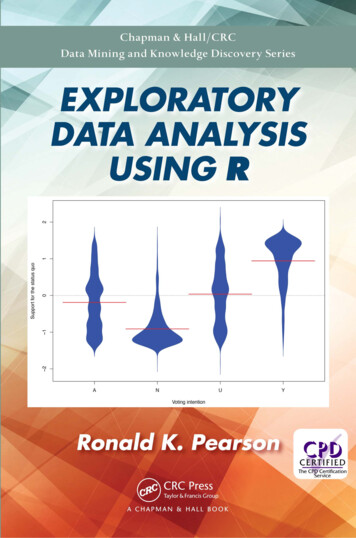
EXPLORATORYDATA ANALYSISUSING R
Chapman & Hall/CRCData Mining and Knowledge SeriesSeries Editor: Vipin KumarComputational Business AnalyticsSubrata DasData ClassificationAlgorithms and ApplicationsCharu C. AggarwalHealthcare Data AnalyticsChandan K. Reddy and Charu C. AggarwalAccelerating DiscoveryMining Unstructured Information for Hypothesis GenerationScott SpanglerEvent MiningAlgorithms and ApplicationsTao LiText Mining and VisualizationCase Studies Using Open-Source ToolsMarkus Hofmann and Andrew ChisholmGraph-Based Social Media AnalysisIoannis PitasData MiningA Tutorial-Based Primer, Second EditionRichard J. RoigerData Mining with RLearning with Case Studies, Second EditionLuís TorgoSocial Networks with Rich Edge SemanticsQuan Zheng and David SkillicornLarge-Scale Machine Learning in the Earth SciencesAshok N. Srivastava, Ramakrishna Nemani, and Karsten SteinhaeuserData Science and Analytics with PythonJesus Rogel-SalazarFeature Engineering for Machine Learning and Data AnalyticsGuozhu Dong and Huan LiuExploratory Data Analysis Using RRonald K. PearsonFor more information about this series please es/CHDAMINODIS
EXPLORATORYDATA ANALYSISUSING RRonald K. Pearson
CRC PressTaylor & Francis Group6000 Broken Sound Parkway NW, Suite 300Boca Raton, FL 33487-2742 2018 by Taylor & Francis Group, LLCCRC Press is an imprint of Taylor & Francis Group, an Informa businessNo claim to original U.S. Government worksPrinted on acid-free paperVersion Date: 20180312International Standard Book Number-13: 978-1-1384-8060-5 (Hardback)This book contains information obtained from authentic and highly regarded sources. Reasonableefforts have been made to publish reliable data and information, but the author and publisher cannotassume responsibility for the validity of all materials or the consequences of their use. The authors andpublishers have attempted to trace the copyright holders of all material reproduced in this publicationand apologize to copyright holders if permission to publish in this form has not been obtained. If anycopyright material has not been acknowledged please write and let us know so we may rectify in anyfuture reprint.Except as permitted under U.S. Copyright Law, no part of this book may be reprinted, reproduced,transmitted, or utilized in any form by any electronic, mechanical, or other means, now known orhereafter invented, including photocopying, microfilming, and recording, or in any informationstorage or retrieval system, without written permission from the publishers.For permission to photocopy or use material electronically from this work, please accesswww.copyright.com (http://www.copyright.com/) or contact the Copyright Clearance Center, Inc.(CCC), 222 Rosewood Drive, Danvers, MA 01923, 978-750-8400. CCC is a not-for-profit organizationthat provides licenses and registration for a variety of users. For organizations that have been granteda photocopy license by the CCC, a separate system of payment has been arranged.Trademark Notice: Product or corporate names may be trademarks or registered trademarks, andare used only for identification and explanation without intent to infringe.Visit the Taylor & Francis Web site athttp://www.taylorandfrancis.comand the CRC Press Web site athttp://www.crcpress.com
ContentsPrefacexiAuthorxiii1 Data, Exploratory Analysis, and R1.1 Why do we analyze data? . . . . .1.2 The view from 90,000 feet . . . . .1.2.1 Data . . . . . . . . . . . . .1.2.2 Exploratory analysis . . . .1.2.3 Computers, software, and R1.3 A representative R session . . . . .1.4 Organization of this book . . . . .1.5 Exercises . . . . . . . . . . . . . .1122471121262 Graphics in R2.1 Exploratory vs. explanatory graphics . . . . . . . .2.2 Graphics systems in R . . . . . . . . . . . . . . . .2.2.1 Base graphics . . . . . . . . . . . . . . . . .2.2.2 Grid graphics . . . . . . . . . . . . . . . . .2.2.3 Lattice graphics . . . . . . . . . . . . . . .2.2.4 The ggplot2 package . . . . . . . . . . . . .2.3 The plot function . . . . . . . . . . . . . . . . . . .2.3.1 The flexibility of the plot function . . . . .2.3.2 S3 classes and generic functions . . . . . . .2.3.3 Optional parameters for base graphics . . .2.4 Adding details to plots . . . . . . . . . . . . . . . .2.4.1 Adding points and lines to a scatterplot . .2.4.2 Adding text to a plot . . . . . . . . . . . .2.4.3 Adding a legend to a plot . . . . . . . . . .2.4.4 Customizing axes . . . . . . . . . . . . . . .2.5 A few different plot types . . . . . . . . . . . . . .2.5.1 Pie charts and why they should be avoided2.5.2 Barplot summaries . . . . . . . . . . . . . .2.5.3 The symbols function . . . . . . . . . . . .2929323333343637374042444448495052535455v.
viCONTENTS2.6.57586164646668703 Exploratory Data Analysis: A First Look3.1 Exploring a new dataset . . . . . . . . . . . . . . . .3.1.1 A general strategy . . . . . . . . . . . . . . .3.1.2 Examining the basic data characteristics . . .3.1.3 Variable types in practice . . . . . . . . . . .3.2 Summarizing numerical data . . . . . . . . . . . . .3.2.1 “Typical” values: the mean . . . . . . . . . .3.2.2 “Spread”: the standard deviation . . . . . . .3.2.3 Limitations of simple summary statistics . . .3.2.4 The Gaussian assumption . . . . . . . . . . .3.2.5 Is the Gaussian assumption reasonable? . . .3.3 Anomalies in numerical data . . . . . . . . . . . . .3.3.1 Outliers and their influence . . . . . . . . . .3.3.2 Detecting univariate outliers . . . . . . . . .3.3.3 Inliers and their detection . . . . . . . . . . .3.3.4 Metadata errors . . . . . . . . . . . . . . . .3.3.5 Missing data, possibly disguised . . . . . . .3.3.6 QQ-plots revisited . . . . . . . . . . . . . . .3.4 Visualizing relations between variables . . . . . . . .3.4.1 Scatterplots between numerical variables . . .3.4.2 Boxplots: numerical vs. categorical variables3.4.3 Mosaic plots: categorical scatterplots . . . . .3.5 Exercises . . . . . . . . . . . . . . . . . . . . . . . 1331351374 Working with External Data4.1 File management in R . . . . . . . . . . . . . . . . . . . .4.2 Manual data entry . . . . . . . . . . . . . . . . . . . . . .4.2.1 Entering the data by hand . . . . . . . . . . . . . .4.2.2 Manual data entry is bad but sometimes expedient4.3 Interacting with the Internet . . . . . . . . . . . . . . . .4.3.1 Previews of three Internet data examples . . . . .4.3.2 A very brief introduction to HTML . . . . . . . . .4.4 Working with CSV files . . . . . . . . . . . . . . . . . . .4.4.1 Reading and writing CSV files . . . . . . . . . . .4.4.2 Spreadsheets and csv files are not the same thing .4.4.3 Two potential problems with CSV files . . . . . . .4.5 Working with other file types . . . . . . . . . . . . . . . iple plot arrays . . . . . . . . .2.6.1 Setting up simple arrays with2.6.2 Using the layout function . .Color graphics . . . . . . . . . . . .2.7.1 A few general guidelines . . .2.7.2 Color options in R . . . . . .2.7.3 The tableplot function . . . .Exercises . . . . . . . . . . . . . . . . . .mfrow. . . . . . . . . . . . . . . . . . .
821851861881881921962012022072112142172212246 Crafting Data Stories6.1 Crafting good data stories . . . . . . . . . . . . . . . . . . .6.1.1 The importance of clarity . . . . . . . . . . . . . . .6.1.2 The basic elements of an effective data story . . . .6.2 Different audiences have different needs . . . . . . . . . . .6.2.1 The executive summary or abstract . . . . . . . . .6.2.2 Extended summaries . . . . . . . . . . . . . . . . . .6.2.3 Longer documents . . . . . . . . . . . . . . . . . . .6.3 Three example data stories . . . . . . . . . . . . . . . . . .6.3.1 The Big Mac and Grande Latte economic indices . .6.3.2 Small losses in the Australian vehicle insurance data6.3.3 Unexpected heterogeneity: the Boston housing 4.5.1 Working with text files . . . . . . . . . .4.5.2 Saving and retrieving R objects . . . . .4.5.3 Graphics files . . . . . . . . . . . . . . .Merging data from different sources . . . . . . .A brief introduction to databases . . . . . . . .4.7.1 Relational databases, queries, and SQL4.7.2 An introduction to the sqldf package .4.7.3 An overview of R’s database support . .4.7.4 An introduction to the RSQLite packageExercises . . . . . . . . . . . . . . . . . . . . .5 Linear Regression Models5.1 Modeling the whiteside data . . . . . . . . .5.1.1 Describing lines in the plane . . . . .5.1.2 Fitting lines to points in the plane . .5.1.3 Fitting the whiteside data . . . . . .5.2 Overfitting and data splitting . . . . . . . . .5.2.1 An overfitting example . . . . . . . . .5.2.2 The training/validation/holdout split5.2.3 Two useful model validation tools . .5.3 Regression with multiple predictors . . . . . .5.3.1 The Cars93 example . . . . . . . . . .5.3.2 The problem of collinearity . . . . . .5.4 Using categorical predictors . . . . . . . . . .5.5 Interactions in linear regression models . . . .5.6 Variable transformations in linear regression .5.7 Robust regression: a very brief introduction .5.8 Exercises . . . . . . . . . . . . . . . . . . . .
viiiCONTENTS7 Programming in R7.1 Interactive use versus programming . . . . . . . . . . . . .7.1.1 A simple example: computing Fibonnacci numbers7.1.2 Creating your own functions . . . . . . . . . . . .7.2 Key elements of the R language . . . . . . . . . . . . . . .7.2.1 Functions and their arguments . . . . . . . . . . .7.2.2 The list data type . . . . . . . . . . . . . . . . .7.2.3 Control structures . . . . . . . . . . . . . . . . . .7.2.4 Replacing loops with apply functions . . . . . . .7.2.5 Generic functions revisited . . . . . . . . . . . . .7.3 Good programming practices . . . . . . . . . . . . . . . .7.3.1 Modularity and the DRY principle . . . . . . . . .7.3.2 Comments . . . . . . . . . . . . . . . . . . . . . . .7.3.3 Style guidelines . . . . . . . . . . . . . . . . . . . .7.3.4 Testing and debugging . . . . . . . . . . . . . . . .7.4 Five programming examples . . . . . . . . . . . . . . . . .7.4.1 The function ValidationRsquared . . . . . . . . .7.4.2 The function TVHsplit . . . . . . . . . . . . . . .7.4.3 The function PredictedVsObservedPlot . . . . .7.4.4 The function BasicSummary . . . . . . . . . . . . .7.4.5 The function FindOutliers . . . . . . . . . . . . .7.5 R scripts . . . . . . . . . . . . . . . . . . . . . . . . . . . .7.6 Exercises . . . . . . . . . . . . . . . . . . . . . . . . . . 772782782792812842858 Working with Text Data8.1 The fundamentals of text data analysis . . . . . . . . . . . .8.1.1 The basic steps in analyzing text data . . . . . . . .8.1.2 An illustrative example . . . . . . . . . . . . . . . .8.2 Basic character functions in R . . . . . . . . . . . . . . . . .8.2.1 The nchar function . . . . . . . . . . . . . . . . . .8.2.2 The grep function . . . . . . . . . . . . . . . . . . .8.2.3 Application to missing data and alternative spellings8.2.4 The sub and gsub functions . . . . . . . . . . . . . .8.2.5 The strsplit function . . . . . . . . . . . . . . . .8.2.6 Another application: ConvertAutoMpgRecords . . .8.2.7 The paste function . . . . . . . . . . . . . . . . . .8.3 A brief introduction to regular expressions . . . . . . . . . .8.3.1 Regular expression basics . . . . . . . . . . . . . . .8.3.2 Some useful regular expression examples . . . . . . .8.4 An aside: ASCII vs. UNICODE . . . . . . . . . . . . . . . .8.5 Quantitative text analysis . . . . . . . . . . . . . . . . . . .8.5.1 Document-term and document-feature matrices . . .8.5.2 String distances and approximate matching . . . . .8.6 Three detailed examples . . . . . . . . . . . . . . . . . . . .8.6.1 Characterizing a book . . . . . . . . . . . . . . . . .8.6.2 The cpus data frame . . . . . . . . . . . . . . . . . 20320322330331336
CONTENTS8.7ix8.6.3 The unclaimed bank account data . . . . . . . . . . . . . 344Exercises . . . . . . . . . . . . . . . . . . . . . . . . . . . . . . . 3539 Exploratory Data Analysis: A Second Look9.1 An example: repeated measurements . . . . . . . . . .9.1.1 Summary and practical implications . . . . . .9.1.2 The gory details . . . . . . . . . . . . . . . . .9.2 Confidence intervals and significance . . . . . . . . . .9.2.1 Probability models versus data . . . . . . . . .9.2.2 Quantiles of a distribution . . . . . . . . . . . .9.2.3 Confidence intervals . . . . . . . . . . . . . . .9.2.4 Statistical significance and p-values . . . . . . .9.3 Characterizing a binary variable . . . . . . . . . . . .9.3.1 The binomial distribution . . . . . . . . . . . .9.3.2 Binomial confidence intervals . . . . . . . . . .9.3.3 Odds ratios . . . . . . . . . . . . . . . . . . . .9.4 Characterizing count data . . . . . . . . . . . . . . . .9.4.1 The Poisson distribution and rare events . . . .9.4.2 Alternative count distributions . . . . . . . . .9.4.3 Discrete distribution plots . . . . . . . . . . . .9.5 Continuous distributions . . . . . . . . . . . . . . . . .9.5.1 Limitations of the Gaussian distribution . . . .9.5.2 Some alternatives to the Gaussian distribution9.5.3 The qqPlot function revisited . . . . . . . . . .9.5.4 The problems of ties and implosion . . . . . . .9.6 Associations between numerical variables . . . . . . .9.6.1 Product-moment correlations . . . . . . . . . .9.6.2 Spearman’s rank correlation measure . . . . . .9.6.3 The correlation trick . . . . . . . . . . . . . . .9.6.4 Correlation matrices and correlation plots . . .9.6.5 Robust correlations . . . . . . . . . . . . . . . .9.6.6 Multivariate outliers . . . . . . . . . . . . . . .9.7 Associations between categorical variables . . . . . . .9.7.1 Contingency tables . . . . . . . . . . . . . . . .9.7.2 The chi-squared measure and Cramér’s V . . .9.7.3 Goodman and Kruskal’s tau measure . . . . . .9.8 Principal component analysis (PCA) . . . . . . . . . .9.9 Working with date variables . . . . . . . . . . . . . . .9.10 Exercises . . . . . . . . . . . . . . . . . . . . . . . . 43844744910 More General Predictive Models10.1 A predictive modeling overview . . . . . . .10.1.1 The predictive modeling problem . .10.1.2 The model-building process . . . . .10.2 Binary classification and logistic regression10.2.1 Basic logistic regression formulation.459459460461462462.
xCONTENTS10.310.410.510.610.710.2.2 Fitting logistic regression models . . . . . .10.2.3 Evaluating binary classifier performance . .10.2.4 A brief introduction to glms . . . . . . . . .Decision tree models . . . . . . . . . . . . . . . . .10.3.1 Structure and fitting of decision trees . . .10.3.2 A classification tree example . . . . . . . .10.3.3 A regression tree example . . . . . . . . . .Combining trees with regression . . . . . . . . . . .Introduction to machine learning models . . . . . .10.5.1 The instability of simple tree-based models10.5.2 Random forest models . . . . . . . . . . . .10.5.3 Boosted tree models . . . . . . . . . . . . .Three practical details . . . . . . . . . . . . . . . .10.6.1 Partial dependence plots . . . . . . . . . . .10.6.2 Variable importance measures . . . . . . . .10.6.3 Thin levels and data partitioning . . . . . .Exercises . . . . . . . . . . . . . . . . . . . . . . .11 Keeping It All Together11.1 Managing your R installation . . . . . .11.1.1 Installing R . . . . . . . . . . . .11.1.2 Updating packages . . . . . . . .11.1.3 Updating R . . . . . . . . . . . .11.2 Managing files effectively . . . . . . . .11.2.1 Organizing directories . . . . . .11.2.2 Use appropriate file extensions .11.2.3 Choose good file names . . . . .11.3 Document everything . . . . . . . . . . .11.3.1 Data dictionaries . . . . . . . . .11.3.2 Documenting code . . . . . . . .11.3.3 Documenting results . . . . . . .11.4 Introduction to reproducible computing11.4.1 The key ideas of reproducibility .11.4.2 Using R Markdown . . . . . . . 7Bibliography539Index544
PrefaceMuch has been written about the abundance of data now available from theInternet and a great variety of other sources. In his aptly named 2007 book Glut[81], Alex Wright argued that the total quantity of data then being produced wasapproximately five exabytes per year (5 1018 bytes), more than the estimatedtotal number of words spoken by human beings in our entire history. And thatassessment was from a decade ago: increasingly, we find ourselves “drowning ina ocean of data,” raising questions like “What do we do with it all?” and “Howdo we begin to make any sense of it?”Fortunately, the open-source software movement has provided us with—atleast partial—solutions like the R programming language. While R is not theonly relevant software environment for analyzing data—Python is another optionwith a growing base of support—R probably represents the most flexible dataanalysis software platform that has ever been available. R is largely based onS, a software system developed by John Chambers, who was awarded the 1998Software System Award by the Association for Computing Machinery (ACM)for its development; the award noted that S “has forever altered the way peopleanalyze, visualize, and manipulate data.”The other side of this software coin is educational: given the availability andsophistication of R, the situation is analogous to someone giving you an F-15fighter aircraft, fully fueled with its engines running. If you know how to fly it,this can be a great way to get from one place to another very quickly. But it isnot enough to just have the plane: you also need to know how to take off in it,how to land it, and how to navigate from where you are to where you want togo. Also, you need to have an idea of where you do want to go. With R, thesituation is analogous: the software can do a lot, but you need to know bothhow to use it and what you want to do with it.The purpose of this book is to address the most important of these questions.Specifically, this book has three objectives:1. To provide a basic introduction to exploratory data analysis (EDA);2. To introduce the range of “interesting”—good, bad, and ugly—featureswe can expect to find in data, and why it is important to find them;3. To introduce the mechanics of using R to explore and explain data.xi
xiiPREFACEThis book grew out of materials I developed for the course “Data Mining UsingR” that I taught for the University of Connecticut Graduate School of Business.The students in this course typically had little or no prior exposure to dataanalysis, modeling, statistics, or programming. This was not universally true,but it was typical, so it was necessary to make minimal background assumptions,particularly with respect to programming. Further, it was also important tokeep the treatment relatively non-mathematical: data analysis is an inherentlymathematical subject, so it is not possible to avoid mathematics altogether,but for this audience it was necessary to assume no more than the minimumessential mathematical background.The intended audience for this book is students—both advanced undergraduates and entry-level graduate students—along with working professionals whowant a detailed but introductory treatment of the three topics listed in thebook’s title: data, exploratory analysis, and R. Exercises are included at theends of most chapters, and an instructor’s solution manual giving completesolutions to all of the exercises is available from the publisher.
AuthorRonald K. Pearson is a Senior Data Scientist with GeoVera Holdings, aproperty insurance company in Fairfield, California, involved primarily in theexploratory analysis of data, particularly text data. Previously, he held the position of Data Scientist with DataRobot in Boston, a software company whoseproducts support large-scale predictive modeling for a wide range of businessapplications and are based on Python and R, where he was one of the authorsof the datarobot R package. He is also the developer of the GoodmanKruskal Rpackage and has held a variety of other industrial, business, and academic positions. These positions include both the DuPont Company and the Swiss FederalInstitute of Technology (ETH Zürich), where he was an active researcher in thearea of nonlinear dynamic modeling for industrial process control, the TampereUniversity of Technology where he was a visiting professor involved in teachingand research in nonlinear digital filters, and the Travelers Companies, where hewas involved in predictive modeling for insurance applications. He holds a PhDin Electrical Engineering and Computer Science from the Massachusetts Institute of Technology and has published conference and journal papers on topicsranging from nonlinear dynamic model structure selection to the problems ofdisguised missing data in predictive modeling. Dr. Pearson has authored orco-authored five previous books, including Exploring Data in Engineering, theSciences, and Medicine (Oxford University Press, 2011) and Nonlinear DigitalFiltering with Python, co-authored with Moncef Gabbouj (CRC Press, 2016).He is also the developer of the DataCamp course on base R graphics.xiii
Chapter 1Data, Exploratory Analysis,and R1.1Why do we analyze data?The basic subject of this book is data analysis, so it is useful to begin byaddressing the question of why we might want to do this. There are at leastthree motivations for analyzing data:1. to understand what has happened or what is happening;2. to predict what is likely to happen, either in the future or in other circumstances we haven’t seen yet;3. to guide us in making decisions.The primary focus of this book is on exploratory data analysis, discussed furtherin the next section and throughout the rest of this book, and this approach ismost useful in addressing problems of the first type: understanding our data.That said, the predictions required in the second type of problem listed aboveare typically based on mathematical models like those discussed in Chapters 5and 10, which are optimized to give reliable predictions for data we have available, in the hope and expectation that they will also give reliable predictions forcases we haven’t yet considered. In building these models, it is important to userepresentative, reliable data, and the exploratory analysis techniques describedin this book can be extremely useful in making certain this is the case. Similarly,in the third class of problems listed above—making decisions—it is importantthat we base them on an accurate understanding of the situation and/or accurate predictions of what is likely to happen next. Again, the techniques ofexploratory data analysis described here can be extremely useful in verifyingand/or improving the accuracy of our data and our predictions.1
2CHAPTER 1. DATA, EXPLORATORY ANALYSIS, AND R1.2The view from 90,000 feetThis book is intended as an introduction to the three title subjects—data, its exploratory analysis, and the R programming language—and the following sectionsgive high-level overviews of each, emphasizing key details and interrelationships.1.2.1DataLoosely speaking, the term “data” refers to a collection of details, recorded tocharacterize a source like one of the following: an entity, e.g.: family history from a patient in a medical study; manufacturing lot information for a material sample in a physical testing application; or competing company characteristics in a marketing analysis; an event, e.g.: demographic characteristics of those who voted for differentpolitical candidates in a particular election; a process, e.g.: operating data from an industrial manufacturing process.This book will generally use the term “data” to refer to a rectangular arrayof observed values, where each row refers to a different observation of entity,event, or process characteristics (e.g., distinct patients in a medical study), andeach column represents a different characteristic (e.g., diastolic blood pressure)recorded—or at least potentially recorded—for each row. In R’s terminology,this description defines a data frame, one of R’s key data types.The mtcars data frame is one of many built-in data examples in R. This dataframe has 32 rows, each one corresponding to a different car. Each of these carsis characterized by 11 variables, which constitute the columns of the data frame.These variables include the car’s mileage (in miles per gallon, mpg), the numberof gears in its transmission, the transmission type (manual or automatic), thenumber of cylinders, the horsepower, and various other characteristics. Theoriginal source of this data was a comparison of 32 cars from model years 1973and 1974 published in Motor Trend Magazine. The first six records of this dataframe may be examined using the head command in R:head(mtcars)##############Mazda RX4Mazda RX4 WagDatsun 710Hornet 4 DriveHornet SportaboutValiantmpg cyl disp hp dratwt qsec vs am gear carb21.06 160 110 3.90 2.620 16.46 0 14421.06 160 110 3.90 2.875 17.02 0 14422.84 108 93 3.85 2.320 18.61 1 14121.46 258 110 3.08 3.215 19.44 1 03118.78 360 175 3.15 3.440 17.02 0 03218.16 225 105 2.76 3.460 20.22 1 031An important feature of data frames in R is that both rows and columns havenames associated with them. In favorable cases, these names are informative,as they are here: the row names identify the particular cars being characterized,and the column names identify the characteristics recorded for each car.
1.2. THE VIEW FROM 90,000 FEET3A more complete description of this dataset is available through R’s built-inhelp facility. Typing “help(mtcars)” at the R command prompt will bring upa help page that gives the original source of the data, cites a paper from thestatistical literature that analyzes this dataset [39], and briefly describes thevariables included. This information constitutes metadata for the mtcars dataframe: metadata is “data about data,” and it can vary widely in terms of itscompleteness, consistency, and general accuracy. Since metadata often providesmuch of our preliminary insight into the contents of a dataset, it is extremelyimportant, and any limitations of this metadata—incompleteness, inconsistency,and/or inaccuracy—can cause serious problems in our subsequent analysis. Forthese reasons, discussions of metadata will recur frequently throughout thisbook. The key point here is that, potentially valuable as metadata is, we cannotafford to accept it uncritically: we should always cross-check the metadata withthe actual data values, with our intuition and prior understanding of the subjectmatter, and with other sources of information that may be available.As a specific illustration of this last point, a popular benchmark dataset forevaluating binary classification algorithms (i.e., computational procedures thatattempt to predict a binary outcome from other variables) is the Pima Indians diabetes dataset, available from the UCI Machine Learning Repository, animportant Internet data source discussed further in Chapter 4. In this particular case, the dataset characterizes female adult members of the Pima Indianstribe, giving a number of different medical status and history characteristics(e.g., diastolic blood pressure, age, and number of times pregnant), along witha binary diagnosis indicator with the value 1 if the patient had been diagnosedwith diabetes and 0 if they had not. Several versions of this dataset are available: the one considered here was the UCI website on May 10, 2014, and it has768 rows and 9 columns. In contrast, the data frame Pima.tr included in R’sMASS package is a subset of this original, with 200 rows and 8 columns. Themetadata available for this dataset from the UCI Machine Learning Repositorynow indicates that this dataset exhibits missing values, but there is also a notethat prior to February 28, 2011 the metadata indicated that there were no missing values. I
Contents Prefacexi Authorxiii 1 Data, Exploratory Analysis, and R 1 1.1 Why do we analyze data? . . . . . . . . .