Exploratory Data Analysis Module II: Leaves And Trees PDF Free Download

1y ago

26 Views

1 Downloads

1.74 MB

21 Pages

Report/dmca

Download PDF

Transcription

Exploratory Data AnalysisModule II: Leaves and TreesDr. Mark WilliamsonDaCCoTAUniversity of North Dakota

Introduction Exploration of datasets to summarize main characteristics Last time: viewing datasummary statisticsbasic graphsbasic tests Coming up: Rational and descriptions Step-by-step examples and assessments Caveats and real-world examples

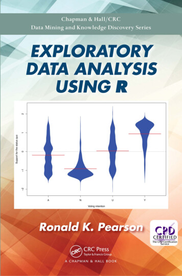
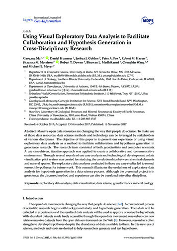
RationalesWhy should we perform exploratory data analysis?1. Get to know your dataCatchIssuesComplexDataCodingIssues2. Save time and effort in the long runFutureVisionDemoResultsReduceMistakes3. Defendable resultsRationaleSummariesAssumptionsSAS: model Temp Weight model Weight TempR: Temp Weight Weight Temp

Descriptions Statistical models – mathematical descriptionof how data conceivably can be produced Parametric data – fits a normal distribution,assumed for many statistical tests Paired data-two measurements notindependent (ex. before/after) Repeated measures-two or moremeasurements not independent (ex. timeintervals) Independent variable-does not depend onanother variable; causative, predictor, X Dependent variable-variable of interest,depends on other variables; response, Y𝒚 𝜷𝟎 𝜷𝟏 𝒙 𝒆

Step-by-step Example 1 Software used: R In the datasets package, I’ll use data set trees Contains the diameter, height, and volume for Black Cherry Trees Research Question: Can we use girth or height to accurately predict volume? Useful because getting volume is difficult--girth and height much easier

Step-by-step Example 11) Look at data print(trees)3 variablesAll numericalNo missing data2) Summary stats summary(trees)Girth Height Volume1 8.3 70 10.32 8.6 65 10.33 8.8 63 10.24 10.5 72 16.45 10.7 81 18.86 10.8 83 19.77 11.0 66 15.68 11.0 75 18.29 11.1 80 22.610 11.2 75 19.911 11.3 79 24.212 11.4 76 21.013 11.4 76 21.414 11.7 69 21.315 12.0 75 19.116 12.9 74 22.217 12.9 85 33.818 13.3 86 27.419 13.7 71 25.720 13.8 64 24.921 14.0 78 34.522 14.2 80 31.723 14.5 74 36.324 16.0 72 38.325 16.3 77 42.626 17.3 81 55.427 17.5 82 55.728 17.9 80 58.329 18.0 80 51.530 18.0 80 51.031 20.6 87 77.0GirthHeightVolumeMin. : 8.30 Min. :63 Min. :10.201st Qu.:11.05 1st Qu.:72 1st Qu.:19.40Median :12.90 Median :76 Median :24.20Mean :13.25 Mean :76 Mean :30.173rd Qu.:15.25 3rd Qu.:80 3rd Qu.:37.30Max. :20.60 Max. :87 Max. :77.00

Step-by-step Example 13) Graphing boxplot(trees) hist(trees Girth) hist(trees Height) hist(trees Volume) trees ln Volume -log(trees Volume) hist(trees ln Volume) qqnorm(trees Volume);qqline(trees Volume) qqnorm(trees ln Volume);qqline(trees ln Volume) plot(trees ln Volume trees Girth) plot(trees ln Volume trees Height) plot(trees Height trees Girth)

Step-by-step Example 14) Simple Tests cor(trees ln Volume, trees Girth) [1] 0.9693838 cor(trees ln Volume, trees Height) [1] 0.6482742[1] 0.5192801 cor(trees Girth, trees Height) lm1 -lm(trees ln Volume trees Girth) summary(lm1) lm2 -lm(trees ln Volume trees Height) summary(lm2)Conclusion: run regressionCall:Call:lm(formula trees ln Volume trees Height)lm(formula trees ln Volume trees Girth)Residuals:Residuals:Min1Q Median3Q MaxMin1QMedianMax 0.58689-0.66691 -0.26539 -0.065553Q0.42608-0.22719 -0.11468 0.02889 0.07930 0.30436Coefficients:Coefficients:Estimate Std. Error t value Pr( t )EstimateStd. Errort value-0.894Pr( t )0.378(Intercept) -0.796520.89053(Intercept)1.118997trees Height0.053540.1040210.01168 10.764.5851.23e-118.03e-05******trees Girth0.1625660.00764721.26 2e-16***----Signif. codes: 0 ‘***’ 0.001 ‘**’ 0.01 ‘*’ 0.05 ‘.’ 0.1 ‘ ’ 1Signif. codes: 0 ‘***’ 0.001 ‘**’ 0.01 ‘*’ 0.05 ‘.’ 0.1 ‘ ’ 1Residual standard error: 0.4076 on 29 degrees of freedomResidualerror:0.1314 on29 degreesof freedomMultiple statistic: 21.02 on 1 and 29 DF, p-value: 8.026e-05F-statistic: 452 on 1 and 29 DF, p-value: 2.2e-16

Assessment 11. What variable is the X variable in the following R equation? What variable is the Y? scatter(leaf number branch number)leaf number is Y (dependent) variablebranch number is X (independent) variable2. Which variable (Fig, Chestnut, and Oak) has the strongest relationship to Apple? Cor(Apple, Fig) ------------- 0.56 Cor(Apple, Chestnut) ----- 0.24 Cor(Apple, Oak) ------------ -0.82Oak has the strongest relationship to Apple3.A) Yes, negative relationshipIs there a relationship between the two variables in the graphs below? If so, what kind?B) Yes, positive relationshipC) NoA)B)C)4.What are two graphs you can use to visualize if data is normally distributed?Histogram, qq-plot5.Is this data normally distributed?Yes, looks to be so

Step-by-step Example 2 Software used: SAS In the sashelp library, I’ll use data set fish Contains the Weight, Length (3 measurements), Height, and Width of 7species of fish caught in Finland Research Question: Is there a width difference between the species of fish?

Step-by-step Example 21) Look at dataPROC PRINT data fish;7 variables Species is categorial nominal, rest arenumerical continuousWeight has a missing value (observation 14)We’ll only use Species and Width (ignore the rest)2) Summary statsPROC UNIVARIATE data fish;var Width;PROC FREQ data fish;tables Species;Obs Species123Mean4Median56Mode ach19Smelt20 Weight Length1 Length2 Length3HeightBasic Statistical MeasuresWidthBream242.023.225.430.0 11.5200 4.0200Bream290.024.026.331.2 12.4800 4.3056LocationVariabilityBream340.023.926.531.1 12.3778 4.69614.417486 Std DeviationBream363.026.329.033.5 12.7300 4.4555Bream430.026.529.034.0 12.4440 5.13404.248500VarianceBream450.026.829.734.7 13.6024 4.9274Bream500.026.829.7 Range34.5 14.1795 5.27853.525000Bream390.027.630.035.0 12.6700 4.6900Range 4.8438Bream450.027.630.0 Interquartile35.1 14.0049Bream500.028.530.736.2 14.2266 4.9594Bream475.028.431.036.2 .2 6.413.75924.36803522.0135Bream.29.532.037.3 13.9129 5.0728116.9246Bream600.029.432.037.2 14.9544 5.1708Bream600.029.432.0 35.2237.2 15.4380 5.580056102Bream700.030.433.038.3 14.8604 5.28541710.69119Bream700.030.433.038.5 14.9380 5.197520139Bream610.030.933.5 12.5838.6 15.6330 5.1338Bream650.031.033.538.7 14.4738 4296.23100.00

Step-by-step Example 23) GraphingPROC SGPLOT data fish;histogram Width;PROC SGPLOT data fish;vbox Width / category Species;

Step-by-step Example 24) Simple TestsDFSum ofSquaresMean SquareF ValuePr F6215.917587035.986264523.47 .0001Error152233.10809371.5336059Corrected Total158449.0256807SourceModelPROC SORT data fish;by Species;Levene's Test for Homogeneity of Width VarianceANOVA of Absolute Deviations from Group MeansPROC UNIVARIATE data fish normal;by Species;var Width;qqplot /normal (mu est sigma est);histogram / normal;PROC GLM data fish;class Species;model Width Species;means Species / hovtest levene(type abs);Conclusion: run modifiedANOVASourceSpeciesErrorDFSum ofSquaresMean SquareF ValuePr F638.65856.443117.04 .000115257.46740.3781

Assessment 21. What variable is the X variable in the following SAS equation? What variable is the Y?model Length SpeciesLength is Y (dependent) variableSpecies is X (independent) variable2.Yes, because the p-value (0.5479) is greater than 0.05, so we fail toreject the hypothesis that the variances are equalBased on the SAS output, is there equal variance?Levene's Test for Homogeneity of Length VarianceANOVA of Absolute Deviations from Group MeansSourceDFSum of SquaresMean SquareF ValuePr 3.Based on the boxplot, would you expectthe categories of cars to have equalvariance? Why or why not?No, the quartile lengths are very different.4.How can the assumption of independent sampling be tested?It can’t. Good sampling design ensures the assumption is met.5.Suppose your data consists of fuel efficiency (miles per gallon) across four different carmakes (Ford, Honda, Nissan, and Dodge). How should you test for normality to run anANOVA (aka, is there a difference in fuel efficiency across makes)?a) check normality over all makes,b) check normality for each make individuallyb)

Caveats and Concerns Normality tests are an art Suggest using histograms and qq-plots over tests for normality There is more than one way of doing things Code output can be confusing Data can be problematic by nature and design Uneven samples sizes Unequal variances

Real World ExamplesZuur, A. F., et al. (2016). "A protocol for conducting and presenting results of regression-typeanalyses." Methods in Ecology and Evolution 7(6): 636-645.

Real World ExamplesAhmed, R., et al. (2020). "United States County-level COVID-19 Death Rates and Case Fatality RatesVary by Region and Urban Status." Healthcare (Basel) 8(3).

Real World ExamplesSchwartz, G. G., et al. (2019). "An exploration of colorectal cancer incidence rates in North Dakota,USA, via structural equation modeling." International Journal of Colorectal Disease 34(9): 15711576.

Summary and Conclusion Exploratory Data Analysis is a necessary first step in understandingyour data and determining how to analyze it Helps to: Get to know your data Save time and effort in the long run End with defendable results Many ways to get it done (R, SAS, SPSS, Excel, etc.) Tune in next time for a plunge into advanced topics of ExploratoryData Analysis in Module III: Deep Dive

Why should we perform exploratory data analysis? 1. Get to know your data 2. Save time and effort in the long run 3. Defendable results Catch Issues Complex Data Coding Future Vision Demo Results Reduce Mistakes Rationale Summaries Assumptions SAS: model Temp W