Transcription
Excel 2016Data analysisCourse objectives: Import dataUse statistical functions in ExcelCreate histogramsGain insights from your dataStudent Training and SupportPhone:(07) 3346 ibrary.uq.edu.au/library-services/training/Service PointsSt Lucia:Hospitals:Gatton:Main desk of the Central, ARMUS and DHESL librariesMain desk of the PACE, Herston and Mater librariesLevel 2, UQ Gatton LibraryStaff Training (Bookings)PhoneEmailWeb(07) 3365 velopmentStaff may contact their trainer with enquiries and feedback related to training content. Please contact Staff Development for bookingenquiries or your local I.T. support for general technical enquiries.Reproduced or adapted from original content provided under Creative Commons license byThe University of Queensland Library
UQ LibraryStaff and Student I.T. TrainingTable of ContentsImporting External Data . 3Importing External Data . 3Importing data from a file . 5Descriptive Statistics . 7Using Descriptive Statistics . 7Statistical Functions . 8Using basic statistical functions in Excel . 8Using Variance and Standard Deviation in Excel . 9Variance and Standard deviation . 9Histograms and Frequency . 11Creating histograms . 11Correlation and Linear Regression . 12Calculate Correlation Co-efficient . 12Create Chart and Linear Regression . 12Forecasting . 15Forecasting . 15T Tests . 16Significance tests . 16ANOVA: Analysis of Variance . 18ANOVA: Analysis of Variance . 18Rank and Percentiles. 19Obtaining your Rank . 19Exercise document:Go to ining/training-resources and click onExcel2016 Data Analysis.xlsx to download. You will also need data.txt from the same location.Save these files on your H:/ drive or to your local machine or a USB drive.Statistical Function definitions can be found 6d659719ffd2 of 19Microsoft Excel 2016: Introduction
UQ LibraryStaff and Student I.T. TrainingImporting External DataData located in compatible external files can be imported into excel without the need to retype allthe information again. Depending on the format of the data you would like to import, differentmethods can be used, including opening and saving in Excel, linking to data, importing data andcopying and pasting data into excel.Importing External DataOpen the spreadsheet Excel2016 Data Analysis.xlsx (which can be found under the Excelsection on the Library Training Resources page. The External Data Link sheet is selected.Importing Data from websitesData from websites and other sources can be imported into Excel if it is in an appropriate format.1. Copy the URL of the web page with the data youwant to import.e.g. World University Rankings on Wikipedia (which can be foundin cell A1 of the External Data Link sheet)https://en.wikipedia.org/wiki/QS World University RankingsNote: For this exercise ignore From Web in the GetExternal Data group. It will bring in the entire webpage and not just a selected table2. Navigate to the Data tab3. Click on New Query (in the Get & Transformgroup)4. From the drop down menu, select From OtherSources From WebThis opens the dialogue box for you to enter the URL of the webpage with the data you want to import5. Paste the URL in the From Web dialogue boxand click OKThe Navigator Pane will open with a list of data that can beimported into excel6. Select the required data set (QS World UniversityRankings – Top 50) on the left pane of theNavigator to preview itNB: You can use the edit button to clean the data beforeimporting7. Select QS World University Rankings – Top 508. Click on Load3 of 19Microsoft Excel: Data Analysis
UQ LibraryStaff and Student I.T. TrainingA connection will be created to the data on the website. This willensure that refreshing your excel file will update the data to thelatest version. Excel will then open a new worksheet with theimported data.Refresh Linked Data9. Click on any cell within the data table10. Click on the Data tab11. Select Refresh AllNB: Refresh all will refresh all connections in the workbook. If youwant to refresh data on a single sheet click RefreshNB: You may get a Microsoft Excel Security Notice aboutconnections to external data sources. You can safely click OK herebut see the section on Considerations when importing data intoExcel below for further information.Considerations when importing data into ExcelMalware / Macros – Unfortunately there are ways to hide malware inside Excel files. This isusually done via “macros” which are little programs that are typically created to do complex orrepetitive tasks. Because hackers have exploited these tools, Microsoft has disabled macros bydefault in Excel. In fact, when you open an Excel file from an untrusted source, you will get asecurity warning like this one. If you are working on data from an unknown or untrusted source,use caution before “Enabling Editing”Some hackers have even learned to use social engineering techniques to try and trick users intoturning macros back on. For example there may be an image in the file that appears blurred with anote that it is for security reasons. The goal is to get you to enable macros so that you can ‘see’the image when, in reality, enabling the macro allows the virus to run. Of course if you have goodanti-virus / anti-malware programs installed, they will go a long way towards mitigating that threat.References within a file or sheet to external dataYou can refer to the contents of cells in another Excel workbook by creating an external reference.An external reference (also called a link) is a reference to a cell or range on a worksheet in anotherExcel workbook, or a reference to a defined name in another workbook. If your data is comingfrom a source beyond your immediate control, you may find that these ‘links’ are broken. If youdon’t have access to the workbooks/worksheets where the underlying data lives, you won’t be ableto use it via the link in the spreadsheet you are currently working on.4 of 19Microsoft Excel: Data Analysis
UQ LibraryStaff and Student I.T. TrainingImporting data from a fileOpen exercise files and enable content1. Open the exercise fileData Analysis Exercises.xlsx andselect the Importing Data & Histogramsworksheet.2. Click on the Enable Content button onthe Security Warning (if necessary)3. If you get a Security Warning dialog box.Click on YesImport data from text file:4. Click the Data tab5. Click From Text (in the Get External Datagroup)6. Locate data analysis.txt7. Click on Import8. Click on Delimited option9. Click Next10. Tick the following options:TabSpaceTreat consecutive delimiters as one11. Click Next5 of 19Microsoft Excel: Data Analysis
UQ LibraryStaff and Student I.T. Training12. Ensure General option is selected13. Click Finish14. Assign data to A 1 in existing worksheet15. Click OK6 of 19Microsoft Excel: Data Analysis
UQ LibraryStaff and Student I.T. TrainingDescriptive StatisticsDescriptive statistics is the discipline of quantitatively (expressed as numbers) describing the mainfeatures of a collection of data. Excel’s Analysis Toolpak add-in offers a variety of features toundertake statistical computations and graphing. Descriptive Statistics is included to providestatistical averages (mean, mode, median), standard error, standard deviation, sample variance,kurtosis and confidence levels of sample data.Using Descriptive Statistics1. Click Data Analysis (at the far right of ribbon)on the Data tab2. Click Descriptive Statistics3. Click OK4. Highlight cells A 1: D 201 for Input Range5. Select Grouped by columns6. Click Labels in first row box7. Click Output Range8. Highlight cell G 1 for Output Range9. Select Summary statistics10. Click OKNB: To obtain descriptive statistics for one groupensure that only one column is selected.7 of 19Microsoft Excel: Data Analysis
UQ LibraryStaff and Student I.T. TrainingStatistical FunctionsUsing basic statistical functions in ExcelTo use Basic Statistical Functions1. Ensure you are on the BasicStatistics worksheet2. Select the Home tab3. Click in cell C144. Click AutoSumCheck the range is (C5:C11)5. Press Enter6. Use Autofill to calculate sum forremaining weeks)7. Calculate with statistical functionsSample size COUNTMean AVERAGEMinimum value MINMaximum value MAXNote: Mean and Average are different terms for thesame thing when dealing with Statistics8. Select cells C14 to C189. Autofill across to fill cells inremaining weeksNB: For quick statistical reference refer to status bar after highlighting a selection of values. Adjust options onstatus bar by right clicking on it and selecting items.8 of 19Microsoft Excel: Data Analysis
UQ LibraryStaff and Student I.T. TrainingUsing Variance and Standard Deviation in ExcelVariance is a measure of the average of the squared difference from the mean.Here is how it is defined manually: Subtract the mean from each value in the data. This gives you a measure of thedistance of each value from the mean.Square each of these distances (so that they are all positive values), and add all of thesquares together.Divide the sum of the squares by the number of values in the data set.(if calculating variance for a sample subtract 1 from the number of values)The standard deviation (σ) is simply a measure of how close the values are to the average. Asmaller number means the values are bunched whilst a larger number indicates values that arespread out.Variance and Standard deviationTo use Variance Function on a sample1. Click in cell C212. Clickbutton in formula bar3. Change category to Statistical4. Click on VAR.S function5. Select range (C5:C11)6. Click on OKTo use Standard Deviation Function on asample1. Click in cell C222. Clickbutton in formula bar3. Change category to Statistical4. Click on STDEV.S function9 of 19Microsoft Excel: Data Analysis
UQ LibraryStaff and Student I.T. Training5. Select range (C5:C11)6. Click on OKRepeat steps above for entire population using range (C5:I11) Click cell C25: Overall Average: AVERAGE(C5:I11) Click cell C26: Overall Variance: VAR.P(C5:I11) Click cell C27: Overall Std Deviation STDEV.P(C5:I11) Click cell C33: Overall Sum SUM(C5:I11)To find WeeklyTotal as a percentage of the Overall Total1. Go to cell C342. Enter C14/C33 in the formula bar3. Press function key F4Note: This will change cell reference C33 to absolute reference C 334. Press enter5. Autofill across (D34:I34)10 of 19Microsoft Excel: Data Analysis
UQ LibraryStaff and Student I.T. TrainingHistograms and FrequencyA histogram is used to display tabulated frequencies of data in graphical form. It is able to showthe proportion of data that fits into specific categories or bins. For example, we may want to findout how many items were of a particular length, e.g. 100mm. Excel provides a Histogram toolwhich is available via the Analysis ToolPak add-in.Creating histogramsUse worksheet “Importing Data & Histograms”Prepare data for a histogram of weights1. Go to cell F192. Type “Bin”3. Go to cell F204. Type 05. Go to cell F216. Type 507. Select F20 and F218. Autofill to display a value of 500 in cell F30Input Range: This is the data that you want to analyse by using the Histogram tool.Bin Range: This represents the intervals that you want the Histogram tool to use for measuring the input data inthe data analysis.9. Click Data Analysis (at the far right of theribbon) on Data tab10. Click on Histogram11. Click OKComplete the dialog box as follows: Input Range A1: A201 Bin Range F 19: F 30 Tick Labels Output Range: I 21 Tick Chart Output12. Click OKTo display the frequencies in Histogram:1. Click on Histogram in worksheet2. Click Data Labels on Add Chart Elementbutton3. Select Outside EndNB: Table with Bin and Frequency headings will appear along with Histogram graph.Resize graph as required.11 of 19Microsoft Excel: Data Analysis
UQ LibraryStaff and Student I.T. TrainingCorrelation and Linear RegressionA correlation is a number between -1 and 1 that summarizes the relationship between twovariables. A correlation close to 1 is strong and positive, whereas a correlation close to -1 is strongbut negative. A zero correlation means there is no relationship between variables.Linear regression is a statistical approach to modelling the relationship between a scalar variabley and one or more explanatory variables denoted X. It can be used for predication or forecasting.Calculate Correlation Co-efficientSelect worksheet “Correlation & Linear Regression”Name cells to find correlation:1. Select cells(B4:B14)2. Click Define Name (near middle ofribbon) on Formulas Tab3. Check name is “Year”4. Click on OK5.6.7.8.Select cells (C4:C14)Click Define Name on Formulas TabCheck name is “Tuition Fees”Click on OKTo calculate correlation co-efficient1. Go to cell B172. Clickbutton in formula bar3. Select Correl function4. In Array 1, type Year (or press F3 for thePaste Name dialog box; Choose thename Year and press OK)5. In Array 2, type Tuition Fees6. Click on OK7. Format cell B17 to 2 decimal placesNote: You will be presented with a strong positive correlation of 0.99 between Year and TuitionFee increasesCreate Chart and Linear RegressionCreate a chart1. Select cells(B4:C14)2. Insert Tab Charts group RecommendedCharts12 of 19Microsoft Excel: Data Analysis
UQ LibraryStaff and Student I.T. Training3. Select ScatterAdd the regression line1. Click Add Chart Element button – Trendline– Linear Trendline2. The Trendline will appear on the chart3. Right click the Trendline4. Choose Format Trendline5. Within Trendline Options .6. Select Checkbox to “Display Equation onChart”Select Checkbox to “Display R-squaredvalue on chart”Note: The equation and R squared value will appeartowards the top right of the chart. If the formulas areobscured by the Trendline, you can move them by selectingthe text box with the formulas and then drag it to where youwant.To Find Regression Summary1. Click on Data Analysis on Data tab (far righton ribbon)2. Select Regression3. Click on OK4.5.6.7.Input Y range, Select C4:C14Input X range, Select B4:B14Output Range, Select A22Click on OKNote: You will be presented with Summary Output whichincludes regression analysis13 of 19Microsoft Excel: Data Analysis
UQ LibraryStaff and Student I.T. TrainingInterpreting results: A demonstrated strong positive correlation:Equation (Y mx c) Y 308.63x 4018.1 Matches the coefficients in regression summaryIntercept indicates the predicted cost of tuition in the Year 2000. This is the line of best fit value not theactual value(the line of best fit value for Y if X 0)X Variable indicates the average increase in in tuition fees year to year approximately 308.6314 of 19Microsoft Excel: Data Analysis
UQ LibraryStaff and Student I.T. TrainingForecastingForecasting is estimating the likelihood of an event taking place in the future, based on availabledata. Statistical forecasting concentrates on using the past to predict the future by identifyingtrends, patterns and business drives within the data to develop a forecast.ForecastingUse worksheet “Correlation & Linear Regression”In Excel the FORECAST function takes raw trendline data, an input (independent variable)and returns the dependent variable1. Click in C 202. Click the Insert Function button3. Select Forecast from the list of functions(search for Forecast in the search box if youcannot see it)4. X, select B205. Known y’s, select C4:C14 (the range nameTuition Fees will appear)6. Known x’s, select B4:B14 (the range nameYear will appear)7.Note how the indicated answer matches the Interceptvalue of the regression analysis8. Click OK9. In cell B20 type 20 to forecast the cost oftuition fees in year 2015 of 19Microsoft Excel: Data Analysis
UQ LibraryStaff and Student I.T. TrainingT TestsTTests are performed when you have two sets of measurements or results from given populationsand you would like to compare them to see if they are significantly different.For example you may have two lists of measurements from the same set of people. The first set ofmeasurements may have been taken in the morning and the second set in the afternoon. This typeof TTest is known as a related TTest or a paired TTest because you have tested the same populationtwice.Alternatively if you had two sets of measurements taken from two sets of people with one set beingin the morning and the other in the afternoon you would have an unpaired or independent TTest.This is because you have tested two different populations.If you are sure about the direction of differences, for example that the morning measurements arefaster than the afternoon then you perform a one tail t test.If you are unsure about the difference between the values perform a two tail t test.A result is called "statistically significant" if the result of the t test comes in at below .05. This is oftenreferred to as the P Value.Significance testsOn the T-Test spreadsheet are two series ofmeasurements.These measurements are paired as they are fromthe same population but taken at different times.1. Select cell B12Using the Insert Function button search for andlocate the T.Test function.Note: The TTest function is still available for compatibilitypurposes with Excel 2007 and below.16 of 19Microsoft Excel: Data Analysis
UQ LibraryStaff and Student I.T. TrainingIn the T.Test Function Arguments dialog box Array1and Array2 are the cell ranges containing the twocolumns of measurements.In this case B3:B10 and C3:C10Tails can be either a 1 or a 2Use 1 if you are sure about the direction of thedifferences.Use 2 if you are unsure about the direction of thedifferences.Type can either be a 1, 2 or 3Use 1 if your data is from a paired population.Use 2 if your data is from an unpaired populationwith an equal variance.Use 3 if your data is from an unpaired populationwith an unequal variance.17 of 19Microsoft Excel: Data Analysis
UQ LibraryStaff and Student I.T. TrainingANOVA: Analysis of VarianceIn its simplest form, ANOVA provides a statistical test of whether or not the means of several groupsare all equal. The ANOVA test is the initial step in identifying factors that are influencing a given dataset. Anova should be performed on 3 or more groups of data.ANOVA: Analysis of VarianceUse worksheet “ANOVA - Rank & percentile”To conduct the one-way ANOVA2. Click on Data Analysis on the Data Tab (farright on ribbon)3. Select Anova: Single Factor4. Click OK.5. Select the input range (A1:C13)(automatically absolute references)6. Click “Labels in first row” option7. Select Output Range (A16)8. Click OK.Note: Descriptive statistics and ANOVA summary table are displayed on screenInterpreting results: In the summary section we can see the mean exam results for each class, But arethese differences statistically significant?There are two types of hypotheses. Null (negative) or Alternative (positive). It is best practice to use nullhypotheses so no personal opinions creep in to the testing statement.A null hypothesis is a default position and can never be proven. Statistically results can only reject or fail toreject the null hypotheses.Null hypotheses are always phrased as a negative statement e.g. There is no real difference between theeffectiveness of lectures, online delivery and video delivery.The test result shows F 0.93 With a critical P-value of .4, the critical F 3.285. Therefore, since the Fstatistic is smaller than the critical value, we fail to reject the null hypothesis. Remember from before the Pvalue is statistically significant if it is below .05. This value of .4 shows there is some connection in the datathough. So, we fail to reject that there is no difference between the effectiveness of lectures, online deliveryand video delivery. These values may be explained by the small sample size. A larger sample of data maygive more statistically significant results. Apparently, the differences we saw in this sample were simply dueto random sampling error.18 of 19Microsoft Excel: Data Analysis
UQ LibraryStaff and Student I.T. TrainingRank and PercentilesPercentile rank means the percentage of scores that fall "at or below" a certain number. Percentilesare most often used for determining the relative standing of an individual in a population or the rankposition of the individual. Percentiles measure position from the bottom.Obtaining your RankUse worksheet “ANOVA - Rank & percentile”1. Click Data Analysis on the Data Tab(far right on ribbon)2. Click Rank and Percentile3. Click OKComplete dialog box:4. Highlight cells A 1: C 13 for InputRangeNB: In this instance, do not merely click on column Aheader as the program will process every row in thespreadsheet.1.2.3.4.In Grouped By, select ColumnsClick Labels in first rowSelect Output Range as M 1Click OKInterpreting results:Point - The location of the value within the original list. This can be used to quickly sort the output table intothe same order of the original list.Original - This is the column containing the original values. This column has the same column name as theoriginal list since we used labels in the first row.Rank - This is the rank of the corresponding number in the list.Percent - This is the numbers percentage rank within the list. This percentage indicates the proportion ofthe list which are below this given number.19 of 19Microsoft Excel: Data Analysis
4 of 19 Microsoft Excel: Data Analysis. A connection will be created to the data on the website. This will ensure that refreshing your excel file will update the data to the latest version. Excel will then open a new worksheet with the imported data. Refresh L