Time Series Forecasting Methods PDF Free Download

2y ago

33 Views

1 Downloads

1.22 MB

43 Pages

Report/dmca

Download PDF

Transcription

IntroductionUnivariate ForecastingConclusionsTime Series Forecasting MethodsNate DerbyStatis Pro Data AnalyticsSeattle, WA, USACalgary SAS Users Group, 11/12/09Nate DerbyTime Series Forecasting Methods1 / 43

IntroductionUnivariate esStrategies2Univariate ForecastingSeasonal Moving AverageExponential SmoothingARIMA3ConclusionsWhich Method?Are Our Results Better?What’s Next?Nate DerbyTime Series Forecasting Methods2 / 43

IntroductionUnivariate esWhat is time series data?What do we want out of a forecast?Long-term or short-term?Broken down into different categories/time units?Do we want prediction intervals?Do we want to measure effect of X on Y ? (scenarioforecasting)What methods are out there to forecast/analyze them?How do we decide which method is best?How can we use SAS for all this?Nate DerbyTime Series Forecasting Methods3 / 43

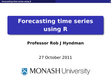
IntroductionUnivariate ForecastingConclusionsObjectivesStrategiesWhat is Time Series Data?Time Series data Data with a pattern (“trend”) over time.Ignore time trend Get wrong results.See my PROC REG paper.Nate DerbyTime Series Forecasting Methods4 / 43

IntroductionUnivariate ForecastingConclusionsObjectivesStrategies!"# "%&'()**&% &#*',)%-' ./.'0'1&2-' .34567 8 9 *)%: *'8 ;' )**&% &#* 600510500110! " " # % # & " '( )* , " ! - " .100410400310300210200/10/000/748 0/710 0/71/ 0/712 0/713 0/714 0/711 0/715 0/716 0/719 0/718 0/750 0/75/ 0/752Nate DerbyTime Series Forecasting Methods5 / 43

IntroductionUnivariate ForecastingConclusionsObjectivesStrategiesBase Data SetNate DerbyTime Series Forecasting Methods6 / 43

IntroductionUnivariate ForecastingConclusionsObjectivesStrategiesWhat do we want out of a Forecast?Long-term:Involves many assumptions! (e.g., global warming)Involves tons of uncertainty.Keynes: “In the long run we are all dead”.We’ll focus on the short term.Different categories?Two strategies for forecasting A, B and C:12Forecast their combined total, then break it down bypercentages.Forecast them separately.Idea: Do (1) unless percentages are unstable.Nate DerbyTime Series Forecasting Methods7 / 43

IntroductionUnivariate ForecastingConclusionsObjectivesStrategiesWhat do we want out of a Forecast?Different time units?Two strategies for forecasting at two different time units (e.g.,daily and weekly):12Forecast weekly, then break down into days by percentages.Forecast daily, then aggregate into weeks.Idea: Idea: Do (1) unless percentages are unstable.Do we want prediction intervals?Prediction interval Interval where data point will be with90/95/99% probability.Yes, we want them!Nate DerbyTime Series Forecasting Methods8 / 43

IntroductionUnivariate ForecastingConclusionsObjectivesStrategiesWhat do we want out of a Forecast?Do we want to measure effect of X on Y ?Ex: Marketing campaign calls to call center.Harder to do, butAllows for scenario forecasting!Idea: Do it, but only with most important X s.Remaining Questions: Basis of this talk:What methods are out there to forecast/analyze them?How do we decide which method is best?How can we use SAS for all this?Methods will require ETS package.Nate DerbyTime Series Forecasting Methods9 / 43

IntroductionUnivariate esTwo stages:Univariate (one variable) forecasting:Forecasts Y from trend alone.Gives us a basic setup.Multivariate (many variables) forecasting:Forecasts Y from trend and other variables X1 , X2 , . . . .Allows for “what if” scenario forecasting.May or may not make more accurate forecasts.Nate DerbyTime Series Forecasting Methods10 / 43

IntroductionUnivariate ForecastingConclusionsSeasonal Moving AverageExponential SmoothingARIMAUnivariate Forecasting - IntroGives us a benchmark for comparing multivariate methods.Could give better forecasts than multivariate.Some methods can be extended to multivariate.Currently three methods:Seasonal moving averageExponential smoothingARIMA(very simple)(simple)(complex)More complex methods, for later on (for me):(promising)(maybe . . . )(forget it!)State spaceBayesianWavelets?Nate DerbyTime Series Forecasting Methods11 / 43

IntroductionUnivariate ForecastingConclusionsSeasonal Moving AverageExponential SmoothingARIMAOnce Again .Q: Why not use PROC REG?Yt β0 β1 Xt ZtA: We can get misleading results (see my PROC REG paper).Nate DerbyTime Series Forecasting Methods12 / 43

IntroductionUnivariate ForecastingConclusionsSeasonal Moving AverageExponential SmoothingARIMASeasonal Moving AverageSimple but sometimes effective!Moving Average:Forecast Average of last n months.Seasonal Moving Average:Forecast Average of last n Novembers.After a certain point, forecast the same for each of sameweekday.Doesn’t allow for a trend.Not based on a model No prediction intervals.Nate DerbyTime Series Forecasting Methods13 / 43

IntroductionUnivariate ForecastingConclusionsSeasonal Moving AverageExponential SmoothingARIMASAS CodeMaking lags in a DATA step (to make the averages) is not fun:Making 4 lags(Brocklebank and Dickey, p. 45)DATA movingaverage;.RETAIN date pass1-pass4;OUTPUT;pass4 pass3;pass3 pass2;pass2 pass1;pass1 pass;RUN;Nate DerbyTime Series Forecasting Methods14 / 43

IntroductionUnivariate ForecastingConclusionsSeasonal Moving AverageExponential SmoothingARIMASAS CodeMuch easier with a trick with PROC ARIMA.Seasonal averaging over past 5 years on that same month:Yt 1(Yt 12 Yt 24 Yt 36 Yt 48 Yt 60 )5Forecasting 3 weeks ahead, seasonal moving averagePROC ARIMA data airline;IDENTIFY var pass noprint;ESTIMATE p ( 12, 24, 36, 48, 60 ) q 0 ar 0.2 0.2 0.2 0.2 0.2noest noconstant noprint;FORECAST lead 12 out foremave id date interval month noprint;RUN;QUIT;Nate DerbyTime Series Forecasting Methods15 / 43

IntroductionUnivariate ForecastingConclusionsSeasonal Moving AverageExponential SmoothingARIMA!"# "%&'()**&% &#*',)%-' ./.'0'1&2-' .34567 8 9 *)%: *'8 ;' )**&% &#* 600510500110! " " # % # & " '( )* , " ! - " .100410400310300210200/10/000/748 0/710 0/71/ 0/712 0/713 0/714 0/711 0/715 0/716 0/719 0/718 0/750 0/75/ 0/752Nate DerbyTime Series Forecasting Methods16 / 43

IntroductionUnivariate ForecastingConclusionsSeasonal Moving AverageExponential SmoothingARIMA!"# "%&'()**&% &#*',)%-' ./.'0'1&2-' .345 6 7 "% '!7 &#) &'8 6 #&2)*9*600510500110! " " # % # & " '( )* , " ! - " .100410400310300210200/10/000/748 0/710 0/71/ 0/712 0/713 0/714 0/711 0/715 0/716 0/719 0/718 0/750 0/75/ 0/752Nate DerbyTime Series Forecasting Methods17 / 43

IntroductionUnivariate ForecastingConclusionsSeasonal Moving AverageExponential SmoothingARIMAExponential Smoothing INotation: ŷt (h) forecast of Y at horizon h, given at time t.Idea 1: Predict Yt h by taking weighted sum of pastobservations:ŷt (h) λ0 yt λ1 yt 1 · · ·Assumes ŷt (h) is constant for all horizons h.Idea 2: Weight recent observations heavier than older ones: λi cαi , 0 α 1 ŷt (h) c yt αyt 1 α2 yt 2 · · ·where c is a constant so that weights sum to 1.Nate DerbyTime Series Forecasting Methods18 / 43

IntroductionUnivariate ForecastingConclusionsSeasonal Moving AverageExponential SmoothingARIMAExponential Smoothing II ŷt (h) c yt αyt 1 α2 yt 2 · · ·Weights are exponentially decaying (hence the name).Choose α by minimizing squared one-step prediction error.Overall:Just a weighted moving average.Can be extended to include trend and seasonality.Prediction intervals? Sort of .Nate DerbyTime Series Forecasting Methods19 / 43

IntroductionUnivariate ForecastingConclusionsSeasonal Moving AverageExponential SmoothingARIMASAS CodeAll done with PROC FORECAST:method expo trend 1 for simple.method expo trend 2 for trend.method winters seasons ( 12 ) for seasonal.Forecasting 3 weeks ahead, exponential smoothingPROC FORECAST data airline method xx interval month lead 12out foreexsm outactual out1step;VAR pass;ID date;RUN;Nate DerbyTime Series Forecasting Methods20 / 43

IntroductionUnivariate ForecastingConclusionsSeasonal Moving AverageExponential SmoothingARIMA!"# "%&'()**&% &#*',)%-' ./.'0'1&2-' .345 "6 7 &'8 9 7 : %&%;") '5 6 : : ; "% ' : #&2)*;*600510500110! " " # % # & " '( )* , " ! - " .100410400310300210200/10/000/748 0/710 0/71/ 0/712 0/713 0/714 0/711 0/715 0/716 0/719 0/718 0/750 0/75/ 0/752Nate DerbyTime Series Forecasting Methods22 / 43

IntroductionUnivariate ForecastingConclusionsSeasonal Moving AverageExponential SmoothingARIMA!"# "%&'()**&% &#*',)%-' ./.'0'1&2-' .3415 6 7 &'8 9 : 5 %&%;") ' 5 5 ; "% '? 5 #&2)*;*600510500110! " " # % # & " '( )* , " ! - " .100410400310300210200/10/000/748 0/710 0/71/ 0/712 0/713 0/714 0/711 0/715 0/716 0/719 0/718 0/750 0/75/ 0/752Nate DerbyTime Series Forecasting Methods23 / 43

IntroductionUnivariate ForecastingConclusionsSeasonal Moving AverageExponential SmoothingARIMA!"# "%&'()**&% &#*',)%-' ./.'0'1&2-' .345 &)*6 %) '7 8 9 6 %&%:") '5 ; 6 6 : "% ' 6 #&2)*:*600510500110! " " # % # & " '( )* , " ! - " .100410400310300210200/10/000/748 0/710 0/71/ 0/712 0/713 0/714 0/711 0/715 0/716 0/719 0/718 0/750 0/75/ 0/752Nate DerbyTime Series Forecasting Methods24 / 43

IntroductionUnivariate ForecastingConclusionsSeasonal Moving AverageExponential SmoothingARIMAExponential Smoothing VIAdvantages:Gives interpretable results (trend seasonality).Gives more weight to recent observations.Disadvantages:Not a model (in the statistical sense).Prediction intervals not (really) possible.Can’t generalize to multivariate approach.Nate DerbyTime Series Forecasting Methods25 / 43

IntroductionUnivariate ForecastingConclusionsSeasonal Moving AverageExponential SmoothingARIMAARIMA IStands for AutoRegressive Integrated Moving Averagemodels.Also known as Box-Jenkins models (Box and Jenkins, 1970).Advantages:Best fit (minimum mean squared forecast error).Generalizes to multivariate approach.Often used in statistical practice.Disadvantages:More complex.Not intuitive at all.Nate DerbyTime Series Forecasting Methods26 / 43

IntroductionUnivariate ForecastingConclusionsSeasonal Moving AverageExponential SmoothingARIMAARIMA IIAssume nonseasonality for now.First, transform, then difference the data {Yt } d times until itis stationary (constant mean, variance), denoted {Yt }.Guesstimate orders p, q through the sample autocorrelation,partial autocorrelation functions.Fit an autoregressive moving average (ARMA) process,orders p and q: · · · φp Yt p Zt θ1 Zt 1 · · · θq Zt qYt φ1 Yt 1φ (Yt ) θ (Zt )iidwhere Zt N(0, σ 2 ), and φ1 , . . . , φp , θ1 , . . . , θq are constants.Through trial and error, repeat above 2 steps until errors “lookgood”.Above is an ARIMA(p, d, q) model.Nate DerbyTime Series Forecasting Methods27 / 43

IntroductionUnivariate ForecastingConclusionsSeasonal Moving AverageExponential SmoothingARIMAConfused Yet?Q: How do we account for seasonality, period s?A: We do almost the exact same thing, except for period s: ,Y Look at {Yt , Yt st 2s , . . .}. Are they stationary? If not,difference D times until they are.Guesstimate orders P and Q similarly to before.Fit “multiplicative ARMA(P, Q)” process, period s: ··· Φ Y Yt Φ1 Yt sP t Ps φ(Yt ) (Zt Θ1 Zt s · · · ΘQ Zt Qs ) θ(Zt )Repeat above 2 steps until all “looks good”.Above is an ARIMA(p, d, q)(P, D, Q)s process.Nate DerbyTime Series Forecasting Methods28 / 43

IntroductionUnivariate ForecastingConclusionsSeasonal Moving AverageExponential SmoothingARIMASAS CodeIf you’re still with me .Yt log(passt ) ARIMA(0, 1, 1) (0, 1, 1)12 :(Yt Yt 1 )(Yt Yt 12 ) (Zt θ1 Zt 1 )(Zt Θ1 Zt 12 )Forecasting 3 weeks ahead, ARIMAPROC ARIMAIDENTIFYESTIMATEFORECASTRUN;QUIT;data airline;var lpass( 1, 12 ) noprint;q ( 1 )( 12 ) noint method ML noprint;lead 12 out forearima id date interval month noprint;Compare with Moving AverageNate DerbyTime Series Forecasting Methods29 / 43

IntroductionUnivariate ForecastingConclusionsSeasonal Moving AverageExponential SmoothingARIMA!"# "%&'()**&% &#*',)%-' ./.'0'1&2-' .34!5 6 7 !'8 9 #&2)*:*600510500110! " " # % # & " '( )* , " ! - " .100410400310300210200/10/000/748 0/710 0/71/ 0/712 0/713 0/714 0/711 0/715 0/716 0/719 0/718 0/750 0/75/ 0/752Nate DerbyTime Series Forecasting Methods31 / 43

IntroductionUnivariate ForecastingConclusionsSeasonal Moving AverageExponential SmoothingARIMABeware the defaults!SAS Codesymbol1 i join c red mode include;symbol2 i join c blue mode include;symbol3 i join c blue l 20 mode include;proc gplot data forearima;plot pass*date 1forecast*date 2l95*date 3u95*date 3 / overlay .;run;quit;Nate DerbyTime Series Forecasting Methods34 / 43

IntroductionUnivariate ForecastingConclusionsWhich Method?Are Our Results Better?What’s Next?Which Method Should be Used?We used three methods, would like to try others later.Q: Which method should be used?Idea: The one that makes the best forecasts!Make k -month-ahead forecasts for the last n months of thedata.For i 1, . . . , n, remove last i months of the data, then makeforecasts for k months in the future.For each method, compare forecasts to actuals.Use forecasts from the method that made the most accurateforecasts.Nate DerbyTime Series Forecasting Methods35 / 43

IntroductionUnivariate ForecastingConclusionsWhich Method?Are Our Results Better?What’s Next?How Do We Judge Forecasts?General standard: Mean Absolute Prediction Error (MAPE):TX forecastt actualt ,MAPE 100 actualtt 1Gives average percentage off (zero is best!).Sometimes different methods best for different horizons.Nate DerbyTime Series Forecasting Methods36 / 43

IntroductionUnivariate ForecastingConclusionsWhich Method?Are Our Results Better?What’s Next?How Do We Do This with SAS?Easy way: Forecast Server or High Performance Forecasting!Follows (and generalizeds) our framework.Implements our methods.Allows us to add our own methods.Harder (but cheaper) way: Program it ourselves.Nate DerbyTime Series Forecasting Methods37 / 43

IntroductionUnivariate ForecastingConclusionsWhich Method?Are Our Results Better?What’s Next?How Do We Do This with SAS?SAS Code ExcerptDATA results;SET all;*merged results, sorted by method;ape3 100*abs( pass - forecast3 )/pass;PROC MEANS data results noprint;BY method;VAR ape3;OUTPUT OUT mapes MEAN( ape3 ) mape3 / noinherit;DATA mapes;SET mapes;IF method 'arima' THEN CALL SYMPUT( 'mapearima', mape3 );IF method 'exsm' THEN CALL SYMPUT( 'mapeexp', mape3 );IF method 'mave' THEN CALL SYMPUT( 'mapemave', mape3 );%LET mapev &mapearima, &mapeexp, &mapemave;DATA null ;IF MIN( &mapev ) &mapearima THEN CALL SYMPUT( 'best', 'arima' );ELSE IF MIN( &mapev ) &mapeexp THEN CALL SYMPUT( 'best', 'exsm' );ELSE IF MIN( &mapev ) &mapemave THEN CALL SYMPUT( 'best', 'mave' );DATA bestforecasts;SET fore&best;RUN;Nate DerbyTime Series Forecasting Methods38 / 43

IntroductionUnivariate ForecastingConclusionsWhich Method?Are Our Results Better?What’s Next?Are Our Overall Forecasts Better?Better forecasts in training set no guarantee of betterforecasts overall!Happily, we often do get better forecasts in general.Nate DerbyTime Series Forecasting Methods39 / 43

IntroductionUnivariate ForecastingConclusionsWhich Method?Are Our Results Better?What’s Next?What’s Next?Multivariate Models!Takes account of holidays/other irregularities.Allows for scenario forecasting!How will we do this?Nate DerbyTime Series Forecasting Methods40 / 43

IntroductionUnivariate ForecastingConclusionsWhich Method?Are Our Results Better?What’s Next?How Will We Do This?One solution: Multivariate ARIMA (transfer models):Yt β0 IXβi Xt i Zt ,Zt ARIMA processi 0Works all right (using PROC ARIMA), butVery complicated to use,Results not very good/useful!One big problem: Parameters are fixed over time.One outlier (e.g., Sept 11) could screw up entire model.If parameters could change over time, model would be (much)more flexible.Nate DerbyTime Series Forecasting Methods41 / 43

IntroductionUnivariate ForecastingConclusionsWhich Method?Are Our Results Better?What’s Next?How Will We Do This?Another solution: State Space (or Hidden Markov) ModelsYt β0t IXβit Xt i Zt ,Zt Normal processi 0Parameters change (slowly) over time.Modeled by separate equation.Complicated, but flexibility makes it worth it.Problem: SAS doesn’t implement it!PROC STATESPACE: Nope! (misleading name)PROC UCM: Closer, but still not there.PROC IML: Can do it, but a fair bit of work.(Almost) no one else (R, S , SPSS) does, either.My next research project!Nate DerbyTime Series Forecasting Methods42 / 43

AppendixFurther ResourcesJohn C. Brocklebank and David A. Dickey.SAS for Forecasting Time Series.SAS Institute, 2003.Chris Chatfield.Time-Series Foreasting.Chapman and Hall, 2000.Nate Derby: http://nderby.orgnderby@sprodata.comNate DerbyTime Series Forecasting Methods43 / 43

What is Time Series Data? Time Series data Data with a pattern (“trend”) over time. Ignore time