WIXLIB

8CONTENTS8.11 Matrix exponential . .8.12 Quadratic form . . . .8.13 Moore-Penrose inverseProblems . . . . . . . . . .9 Dynamical systems9.1 Paradigm problems . . . . . . . . . . . . . . . .9.1.1 Autonomous example . . . . . . . . . . .9.1.2 Non-autonomous example . . . . . . . .9.2 General theory . . . . . . . . . . . . . . . . . .9.3 Iterated maps . . . . . . . . . . . . . . . . . . .9.4 High order scalar differential equations . . . . .9.5 Linear systems . . . . . . . . . . . . . . . . . .9.5.1 Homogeneous equations with constant A9.5.1.1 N eigenvectors . . . . . . . . .9.5.1.2 N eigenvectors . . . . . . . .9.5.1.3 Summary of method . . . . . .9.5.1.4 Alternative method . . . . . . .9.5.1.5 Fundamental matrix . . . . . .9.5.2 Inhomogeneous equations . . . . . . . .9.5.2.1 Undetermined coefficients . . .9.5.2.2 Variation of parameters . . . .9.6 Non-linear systems . . . . . . . . . . . . . . . .9.6.1 Definitions . . . . . . . . . . . . . . . . .9.6.2 Linear stability . . . . . . . . . . . . . .9.6.3 Lyapunov functions . . . . . . . . . . . .9.6.4 Hamiltonian systems . . . . . . . . . . .9.7 Differential-algebraic systems . . . . . . . . . .9.7.1 Linear homogeneous . . . . . . . . . . .9.7.2 Non-linear . . . . . . . . . . . . . . . . .9.8 Fixed points at infinity . . . . . . . . . . . . . .9.8.1 Poincaré sphere . . . . . . . . . . . . . .9.8.2 Projective space . . . . . . . . . . . . . .9.9 Fractals . . . . . . . . . . . . . . . . . . . . . .9.9.1 Cantor set . . . . . . . . . . . . . . . . .9.9.2 Koch curve . . . . . . . . . . . . . . . .9.9.3 Menger sponge . . . . . . . . . . . . . .9.9.4 Weierstrass function . . . . . . . . . . .9.9.5 Mandelbrot and Julia sets . . . . . . . .9.10 Bifurcations . . . . . . . . . . . . . . . . . . . .9.10.1 Pitchfork bifurcation . . . . . . . . . . .9.10.2 Transcritical bifurcation . . . . . . . . .CC BY-NC-ND. 29 July 2012, Sen & 6450452452453453454454455456457

9CONTENTS9.10.3 Saddle-node bifurcation .9.10.4 Hopf bifurcation . . . . .9.11 Lorenz equations . . . . . . . . .9.11.1 Linear stability . . . . . .9.11.2 Non-linear stability: center9.11.3 Transition to chaos . . . .Problems . . . . . . . . . . . . . . . . . . . . . . . . . . . . . . . . . . . . . . . . . . . . . . . . . . . . . . . . . . . .manifold projection. . . . . . . . . . . . . . . . . . . . . . .10 Appendix10.1 Taylor series . . . . . . . . . . . . . . . . . . . . . . . .10.2 Trigonometric relations . . . . . . . . . . . . . . . . . .10.3 Hyperbolic functions . . . . . . . . . . . . . . . . . . .10.4 Routh-Hurwitz criterion . . . . . . . . . . . . . . . . .10.5 Infinite series . . . . . . . . . . . . . . . . . . . . . . .10.6 Asymptotic expansions . . . . . . . . . . . . . . . . . .10.7 Special functions . . . . . . . . . . . . . . . . . . . . .10.7.1 Gamma function . . . . . . . . . . . . . . . . .10.7.2 Beta function . . . . . . . . . . . . . . . . . . .10.7.3 Riemann zeta function . . . . . . . . . . . . . .10.7.4 Error functions . . . . . . . . . . . . . . . . . .10.7.5 Fresnel integrals . . . . . . . . . . . . . . . . . .10.7.6 Sine-, cosine-, and exponential-integral functions10.7.7 Elliptic integrals . . . . . . . . . . . . . . . . .10.7.8 Hypergeometric functions . . . . . . . . . . . .10.7.9 Airy functions . . . . . . . . . . . . . . . . . . .10.7.10 Dirac δ distribution and Heaviside function . . .10.8 Total derivative . . . . . . . . . . . . . . . . . . . . . .10.9 Leibniz’s rule . . . . . . . . . . . . . . . . . . . . . . .10.10Complex numbers . . . . . . . . . . . . . . . . . . . . .10.10.1 Euler’s formula . . . . . . . . . . . . . . . . . .10.10.2 Polar and Cartesian representations . . . . . . .10.10.3 Cauchy-Riemann equations . . . . . . . . . . .Problems . . . . . . . . . . . . . . . . . . . . . . . . . . . 94494496497499CC BY-NC-ND.29 July 2012, Sen & Powers.

10CC BY-NC-ND. 29 July 2012, Sen & Powers.CONTENTS

PrefaceThese are lecture notes for AME 60611 Mathematical Methods I, the first of a pair of courseson applied mathematics taught in the Department of Aerospace and Mechanical Engineeringof the University of Notre Dame. Most of the students in this course are beginning graduatestudents in engineering coming from a variety of backgrounds. The course objective is tosurvey topics in applied mathematics, including multidimensional calculus, ordinary differential equations, perturbation methods, vectors and tensors, linear analysis, linear algebra,and non-linear dynamic systems. In short, the course fully explores linear systems and considers effects of non-linearity, especially those types that can be treated analytically. Thecompanion course, AME 60612, covers complex variables, integral transforms, and partialdifferential equations.These notes emphasize method and technique over rigor and completeness; the studentshould call on textbooks and other reference materials. It should also be remembered thatpractice is essential to learning; the student would do well to apply the techniques presentedby working as many problems as possible. The notes, along with much information on thecourse, can be found at http://www.nd.edu/ powers/ame.60611. At this stage, anyone isfree to use the notes under the auspices of the Creative Commons license below.These notes have appeared in various forms over the past years. An especially generaltightening of notation and language, improvement of figures, and addition of numerous smalltopics was implemented in 2011. Fall 2011 students were also especially diligent in identifyingadditional areas for improvement. We would be happy to hear further suggestions from you.Mihir SenMihir.Sen.1@nd.eduhttp://www.nd.edu/ msenJoseph M. Powerspowers@nd.eduhttp://www.nd.edu/ powers\Notre Dame, Indiana; USA CCBY:29 July 2012The content of this book is licensed under Creative Commons Attribution-Noncommercial-No DerivativeWorks 3.0.11

12CC BY-NC-ND. 29 July 2012, Sen & Powers.CONTENTS

Chapter 1Multi-variable calculussee Kaplan, Chapter 2: 2.1-2.22, Chapter 3: 3.9,Here we consider many fundamental notions from the calculus of many variables.1.1Implicit functionsThe implicit function theorem is as follows:TheoremFor a given f (x, y) with f 0 and f / y 6 0 at the point (xo , yo ), there corresponds aunique function y(x) in the neighborhood of (xo , yo ).More generally, we can think of a relation such asf (x1 , x2 , . . . , xN , y) 0,(1.1)also written asf (xn , y) 0,n 1, 2, . . . , N,(1.2)in some region as an implicit function of y with respect to the other variables. We cannothave f / y 0, because then f would not depend on y in this region. In principle, we canwritey y(x1 , x2 , . . . , xN ),ory y(xn ), n 1, . . . , N,(1.3)if f / y 6 0.The derivative y/ xn can be determined from f 0 without explicitly solving for y.First, from the definition of the total derivative, we havedf f f f f fdx1 dx2 . . . dxn . . . dxN dy 0. x1 x2 xn xN y(1.4)Differentiating with respect to xn while holding all the other xm , m 6 n, constant, we get f f y 0, xn y xn13(1.5)

14CHAPTER 1. MULTI-VARIABLE CALCULUSso that f yn, x f xn y(1.6)which can be found if f / y 6 0. That is to say, y can be considered a function of xn if f / y 6 0.Let us now consider the equationsf (x, y, u, v) 0,g(x, y, u, v) 0.(1.7)(1.8)Under certain circumstances, we can unravel Eqs. (1.7-1.8), either algebraically or numerically, to form u u(x, y), v v(x, y). The conditions for the existence of such a functionaldependency can be found by differentiation of the original equations; for example, differentiating Eq. (1.7) givesdf f f f fdx dy du dv 0. x y u v(1.9)Holding y constant and dividing by dx, we get f u f v f 0. x u x v x(1.10)Operating on Eq. (1.8) in the same manner, we get g g u g v 0. x u x v x(1.11)Similarly, holding x constant and dividing by dy, we get f u f v f 0, y u y v y g g u g v 0. y u y v y(1.12)(1.13)Equations (1.10,1.11) can be solved for u/ x and v/ x, and Eqs. (1.12,1.13) can be solvedfor u/ y and v/ y by using the well known Cramer’s1 rule; see Eq. (8.93). To solve for u/ x and v/ x, we first write Eqs. (1.10,1.11) in matrix form: f u g u f v g v u 1 x v x f x g x .(1.14)Gabriel Cramer, 1704-1752, well-traveled Swiss-born mathematician who did enunciate his well knownrule, but was not the first to do so.CC BY-NC-ND. 29 July 2012, Sen & Powers.

151.1. IMPLICIT FUNCTIONSThus, from Cramer’s rule we have u x f x g x f u g u f v g v f v g v (f,g) (x,v) (f,g) (u,v) f u g u f u g u v x, f x g x f v g v (f,g) (u,x) (f,g) . (u,v)(1.15)In a similar fashion, we can form expressions for u/ y and v/ y: u y f y g y f u g u f v g v f v g v (f,g) (y,v) (f,g) (u,v) f u g u f u g u v y, f y g y f v g v (f,g) (u,y) (f,g) (u,v).Here we take the Jacobian2 matrix J of the transformation to be defined as f f u v.J g g u(1.16)(1.17) vThis is distinguished from the Jacobian determinant, J, defined asJ det J (f, g) (u, v) f u g u f v g v.(1.18)If J 6 0, the derivatives exist, and we indeed can form u(x, y) and v(x, y). This is thecondition for existence of implicit to explicit function conversion.Example 1.1Ifx y u6 u v 0,(1.19)xy uv 1,(1.20)find u/ x.Note that we have four unknowns in two equations. In principle we could solve for u(x, y) andv(x, y) and then determine all partial derivatives, such as the one desired. In practice this is not alwayspossible; for example, there is no general solution to sixth order polynomial equations such as we havehere.Equations (1.19,1.20) are rewritten asf (x, y, u, v)x y u6 u v 0,(1.21)g(x, y, u, v) xy uv 1 0.(1.22)2Carl Gustav Jacob Jacobi, 1804-1851, German/Prussian mathematician who used these quantities,which were first studied by Cauchy, in his work on partial differential equations.CC BY-NC-ND.29 July 2012, Sen & Powers.

16CHAPTER 1. MULTI-VARIABLE CALCULUSUsing the formula from Eq. (1.15) to solve for the desired derivative, we get u x f x g x f u g u f v g v f v g v.(1.23)Substituting, we get 1 1 y u uy u . xu(6u5 1) v6u5 1 1vu(1.24)v 6u6 u,(1.25)Note whenthat the relevant Jacobian determinant is zero; at such points we can determine neither u/ x nor u/ y; thus, for such points we cannot form u(x, y).At points where the relevant Jacobian determinant (f, g)/ (u, v) 6 0 (which includes nearly all ofthe (x, y) plane), given a local value of (x, y), we can use algebra to find a corresponding u and v, whichmay be multivalued, and use the formula developed to find the local value of the partial derivative.1.2Functional dependenceLet u u(x, y) and v v(x, y). If we can write u g(v) or v h(u), then u and v are saidto be functionally dependent. If functional dependence between u and v exists, then we canconsider f (u, v) 0. So, f u f v 0, u x v x f u f v 0. u y v y(1.26)(1.27)In matrix form, this is u x u y v x v y f u f v 0 .0(1.28)Since the right hand side is zero, and we desire a non-trivial solution, the determinant of thecoefficient matrix must be zero for functional dependency, i.e. u x u yCC BY-NC-ND. 29 July 2012, Sen & Powers. v x v y 0.(1.29)

171.2. FUNCTIONAL DEPENDENCENote, since det J det JT , that this is equivalent to u x v xJ u y v y (u, v) 0. (x, y)(1.30)That is, the Jacobian determinant J must be zero for functional dependence.Example 1.2Determine ifuvw y z,(1.31)2 x 2z , x 4yz 2y 2 ,(1.32)(1.33)are functionally dependent.The determinant of the resulting coefficient matrix, by extension to three functions of three variables, is (u, v, w) (x, y, z) u x v x w x u y v y w y u z v z w z u x u y u z 0 11 01 4z v x v y v z w x w y w z,(1.34)1 4(y z) , 4y(1.35) ( 1)( 4y ( 4)(y z)) (1)(4z), 4y 4y 4z 4z, 0.(1.36)(1.37)(1.38)So, u, v, w are functionally dependent. In fact w v 2u2 .Example 1.3Letx y zx y z 2 2xz22 0, 1.(1.39)(1.40)Can x and y be considered as functions of z?If x x(z) and y y(z), then dx/dz and dy/dz must exist. If we takef (x, y, z) g(x, y, z) f f fdz dx dy df z x yx y z 0,x2 y 2 z 2 2xz 1 0,(1.41)(1.42)0,(1.43)CC BY-NC-ND.29 July 2012, Sen & Powers.

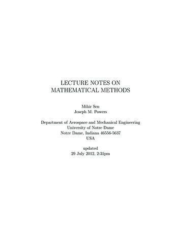
18CHAPTER 1. MULTI-VARIABLE CALCULUSdg g g gdz dx dy z x y f dx f dy f z x dz y dz g g dx g dy z x dz y dz f f dx x ydz g gdy x ydz0,(1.44)0,(1.45)0, (1.46) f z g z ,(1.47)Tthen the solution matrix (dx/dz, dy/dz) can be obtained by Cramer’s rule:dx dzdydz f z g z f y g y f y g y f x g x f x g x f x g x 11 (2z 2x) 2y 2y 2z 2x 1, 2y 2x 2z112x 2z 2y f z g z f y g y 1 (2z 2x)0 .2y 2x 2z112x 2z 2y12x 2z(1.48)(1.49)Note here that in the expression for dx/dz that the numerator and denominator cancel; there is nospecial condition defined by the Jacobian determinant of the denominator being zero. In the second,dy/dz 0 if y x z 6 0, in which case this formula cannot give us the derivative.Now, in fact, it is easily shown by algebraic manipulations (which for more general functions arenot possible) thatx(z) y(z) 2, z 2 2 .2(1.50)(1.51)This forms two distinct lines in x, y, z space. Note that on the lines of intersection of the two surfacesthat J 2y 2x 2z 2 2, which is never indeterminate.The two original functions and their loci of intersection are plotted in Fig. 1.1. It is seen that thesurface represented by the linear function, Eq. (1.39), is a plane, and that represented by the quadraticfunction, Eq. (1.40), is an open cylindrical tube. Note that planes and cylinders may or may notintersect. If they intersect, it is most likely that the intersection will be a closed arc. However, whenthe plane is aligned with the axis of the cylinder, the intersection will be two non-intersecting lines;such is the case in this example.Let us see how slightly altering the equation for the plane removes the degeneracy. Take now5x y zx y z 2 2xz2 0, 1.2(1.52)(1.53)Can x and y be considered as functions of z? If x x(z) and y y(z), then dx/dz and dy/dz mustexist. If we takef (x, y, z) 5x y z 0,222g(x, y, z) x y z 2xz 1 0,CC BY-NC-ND. 29 July 2012, Sen & Powers.(1.54)(1.55)

191.3. COORDINATE TRANSFORMATIONS-12x01y101-10.5-210 z-0.50.5z-10.500 y-0.5-0.5-1-1-0.500.5x1Figure 1.1: Surfaces of x y z 0 and x2 y 2 z 2 2xz 1, and their loci of intersection.Tthen the solution matrix (dx/dz, dy/dz) is found as before: f z gdx f zdz xdy dz f x g x f x g x g x f z g z f y g y f y g y f y g y 11 (2z 2x) 2y 2y 2z 2x, 10y 2x 2z512x 2z 2y(1.56) 1 (2z 2x)

These are lecture notes for AME 60611 Mathematical Methods I, the first of a pair of courses on applied mathematics taught in the Department of Aerospace and Mechanical Engineering of the University of Notre Dame. Most of the students in this course are beginning graduate stud