Transcription
Urban Network Analysis Toolboxfor Rhinoceros 3DHELPversion 5.10.10.3 R5RS10
City Form Lab, 2015Andres Sevtsuk; Raul KalvoContact:cityformlab[at]mit.eduSingapore University of Technology & Design in collaboration with MIT8 Somapah RdSingapore, 487372T: 65-64994557LicenseThe Urban Network Analysis Toolbox for Rhinoceros 3D is distributed by the City FormLab and can be used under the License of Creative Commons Attribution-NoDerivatives4.0 International. For more information, alcode1
CONTENTS1Introduction .22Installation .32.1Download .33Graphic User Interface . 54Bibliography . 271INTRODUCTIONUrban Network Analysis (UNA) offers powerful methods for assessing distances,accessibilities and encounters between people or places along spatial networks. Thenew UNA Rhino toolbox makes urban network analysis available in Rhino 5, adding anumber of new features and functionalities. The UNA Rhino toolbox was developed inorder to make spatial network analysis tools available to architects, designers andplanners who do not have access to GIS and typically work on designs in Rhino. HavingUNA metrics in Rhino, not only allows one to analyze how a specific spatial networkperforms, but to also incorporate the analysis into a fast and iterative design process,where networks can be designed, evaluated and redesigned in seamless cycles to rapidlyimprove the outcome.The UNA Rhino toolbox is significantly faster that its GIS counterpart, which has beenavailable as a plugin for ArcGIS since 2012. Users also have an ability to rapidly createand edit networks from any Rhino curve objects, making network design and redesignsimple and intuitive. The analytic options available to the user have expanded, givingyou more precise control to analyze exactly what you need for every unique spatialnetwork problem.The toolbox is in beta version. It is still in development and we look forward to yourfeedback and suggestions in making it better for day-tod-day design and researchpractice.The bibliography attached to the bottom of this tutorial includes a set of articles andbooks on the subject. A short introductory video about the Urban Network Analysis canbe found online at: http://vimeo.com/447285302
2 INSTALLATION2.1DOWNLOADBefore you install the UNA toolbar, make sure you have Rhino version 5 and the latestupdates from McNeel installed. You can install the updates by opening Rhino and goingto help check for updates.Download the UNA Toolbox folder from the following Dropbox olboxYou should see the “UNAToolbox.rhi” file. Run it and navigate through the installationsteps.Note, that with some recent McNeel updates the .rhi installer for UNA may not berecognized as a program on windows. This is a known Rhino bug that McNeel is awareof. You can still install the UNA toolbox in one of two ways:a) drag and drop the *.rhi installer file into an open Rhino window.b) reassociate the *.rhi file in Windows again with C:\Program Files\Rhinoceros 5(64-bit)\System\x64\rhiexec.exeOnce installed, you may see the UNA toolbar appear automatically in Rhino. If it doesnot appear automatically, then in Rhino, go to Tools Toolbars tab and make sure youcheck the box next for UNA. Click “OK”.3
Now you should see a new toolbar in Rhino that looks like this:These are the tools that enable Urban Network Analysis in Rhino. You can also activateeach of the tools from the Command Line. UNA tools typically start with the “una ”followed by the tool name for each function.4
3 GRAPHIC USER INTERFACEThe GUI is divided into five sections, providing attribute editing, data import/export,network setup, analysis, and graphic settings functionality respectively.The first set of the tools (Tools 1-7 from the left) deal with assigning objects attributes,which are optional to the analysis.The UNA Toolbox for Rhino utilizes “attributes” to give properties to origin anddestination objects, such as names, numeric or weights. These attributes are analogousto Attribute Tables in ArcGIS shapefiles. An object can have any number of attributes.However, unlike ArcGIS, the Rhino attributes are not stored as a table, but rather as adictionary, where the key indicates the attribute name and values indicate attributesvalues. Attributes can be either numeric or text based.1. Add Text Attribute to ObjectsAttributes allow you to distinguish spatial objects from one another by givingthem unique properties that correspond to their real world characteristics.Assigning a Text Attribute to geometric objects in Rhino could, for instance, beused to designate a “Business name” or “Cleanliness Rating” in the range of “A”,“B”, “C” etc. Text attributes you enter can also be used as an IDs or any otherdescriptive fields that may be helpful in your analysis. Text attributes can not beused as weights in the analysis.The tool allows you to select one or more objects at a time and then prompts for:Attribute Name Attribute Value.Your chosen “Attribute Name” is a dictionary key, analogous to a column name ina table. The “Text Value” is the value that corresponds to the Attribute (e.g.dictionary entry or row value in a table).2. Add Numeric Attribute to ObjectsThis tools allows you to add a Numeric Attribute to geometric objects in Rhino.Numeric attributes are particularly useful for spatial network analysis as they5
allow you to “weigh” the analysis according to each object’s value. A “NumericAttribute” could, for instance, indicate the “Number of Floors” in a building, the“Area” of a space, the “Number of Employees” in a business etc. The attribute youprovide can later be used as a “weight” in your analysis. The tool allows you toselect one or more objects at a time for inputting these attributes and thenprompts for:Attribute Name Attribute Value.Your chosen “Attribute Name” is dictionary key, analogous to a column name in atable. The “Text Value” is the value that corresponds to this Attribute (e.g.dictionary entry or row value in a table). Note that the numeric input may be aninteger or a decimal point number, negative or positive.3. Add Tag Attribute to ObjectsThis tool allows you to add a tag name to chosen objects. After selecting theobjects, the tool prompts you for the attribute name by prompting “tag :” onthe command line. Assign the tab name you want to use on the command lineand press enter. The tag you enter is simply a name that doesn’t contain anyvalues, as opposed to the text or number values in the previous two tools.4. Remove Attribute from ObjectsThis tool allows you to get rid of some previously added attributes from chosenobjects. If you choose all objects in the scene and apply this tool, then all objectswill lose the tags you specify.After selecting the objects, the tool prompts you for the tag name by asking “Tag:“ on the command line. Type in the tag name that you want to remove. Note thatyou cannot remove GUID, which is a unique ID for each Rhino object.5. Save Result as WeightThis tool allows you to one result at a time to the object attributes, optionallyassigning it a custom column name in the table.6. Show Attribute Tree6
This tool allows you to see what attributes objects carry. The attributes arestructured as a tree, showing the name of the attribute, value type (e.g. string,double, integer etc.) and value. Note that every geometric object in Rhinoautomatically carries a unique GUID. This is the first attribute you see in anyobject’s Attribute Tree. In the image below, the rectangle that is selected has aGUID, a Text string Attribute called “Name” with a value of “rectangle” and aNumeric Attribute called “Area” with a value of “13106.5972”.The “Load Selected” button allows you to pull up the attributes of only selectedobjects. The “Load” button lists the attributes of all objects in your Rhino scene.Note that if you have a lot of objects, this list can be very long and hard to follow,loading selected attributes is typically more practical.The next section of tools Next we turn to tools that allow you to import or exportdata from/to UNA network objects.7
7. Import pointsThe import points tool can be used to bring in origin or destination point datawith attributes from GIS or other table files to Rhino. The tables you import mayinclude X,Y and optionally Z coordinates, which will be drawn as points in Rhino.All other columns from the original table are brought along as attributes to thepoints in Rhino.Note that there are some restriction in how your table columns can be named sothat Rhino can recognize them as attribute names: Spaces in column names are automatically ignored (e.g. “My Name” isconverted to “MyName”).Underscores that form the first character in a column name areautomatically removed.column names can contain numbers but the entire name may not be anumber.A couple of names are reserved for internal UNA processes – “none” and“count” may not be used as column names.8. Import TableThis tool allows you to bring in a table of attributes that may pre-exist or thatmay be available as part of some other dataset you have in GIS, Excel, etc. Inorder to import any of such attribute tables, you will need to first convert the preexisting tables into either “tab separated values” (“tsv”) or comma separatedvalues (“csv”). The tool can only accept these formats. It is very common to havedata in an Excel sheet, which allows you to save to either a “Text (Tab Delimited)(*.txt)” or “CSV (Comma Delimited) (*.csv)” formats. The default format is “tsv”.Click on the “Format tsv” option in the command line if you want to switch to“csv”.Click on the “File” option in the command to browse to the file you want toimport.The “Geometry all” default option will attempt to match the importedattributes to all objects in your Rhino file. You can also choose to only try to join8
attributes to selected objects, by changing this to “Geometry selected” andclicking on this value in the command line. This will prompt you for an objectselection.The “UpdateWeights On” default option requests that your newly importedattribute values will automatically be available as weights for UNA analyses. Ifweights with the same name already exist on Rhino objects, they will be rewritten as part of the ImportTable process.9. ExportThis tool allows you to export the attributes you have added manually or obtainedwhen Rhino UNA analysis tools, into a table. The command line offers a fewoptions. You can change formats between tab separated values “tsv” and commaseparated values “csv”, and you can choose to either output the entire table toclipboard (memory) or to a file. If you output to the default memory, then youcan simply “paste” in Excel and the exported values are dropped into a table. Thiscan be useful if you would like to manipulate object weights or join the attributeswith additional indicators in Excel.Next we turn to tools that allow you to construct spatial networks and add/removeorigins and destinations on the networks.10.Add Curves to NetworkThe way spatial networks are represented in the Rhino UNA toolbox is similar tothe ArcGIS UNA toolbox (if you happen to have used it). Any network analysisrequires at least two user inputs: first, an input analysis network and second,input locations. If you have been using our GIS UNA toolbox may recall thatcreating new network datasets (ND) in ArcGIS requires multiple steps and isdifficult to automate. Furthermore, at the start of calculating each centralityanalysis in ArcGIS, an “adjacency matrix” is calculated, among the input pointson the network. Depending on the size of the dataset, this can take substantialtime in GIS. These two procedures – creating a network and creating anadjacency matrix – are substantially more efficient in Rhino, as explained below.The Add Curves to Network tool asks you to select curves that you want to buildyour network out of. Select all the curves you want to involve in the network and9
press enter. This will automatically turn the selected curves into a network andbuild an adjacency matrix that is used for analysis later.Note that through a left click, this tool also enables you to add more curves to thenetwork you have already built. If some of the curves you might be adding to apre-existing network are already part of the network, their GUIDs will berecognized and they will not be double represented. Right clicking the tool, on theother hand, allows you to remove curves from an existing network.In order for network analyses to work, network curves need to provide continuitybetween the “input locations” you analyze. If your network curves do not share acommon end node, then the “input locations” found on different networksegments will not be topologically connected to each other. If one curve ends ontop of another, but the latter does not have a node at the intersection point, thentopologically there will not be a continuity between the two curves. Curves thatintersect without sharing a common node can be used to model 3d overpasses orunderpasses.The tool can accept any kinds of curves to participate in networks – lines,polylines, curves, arcs, etc. Networks of these curves can either be planar (2D) orthree-dimensional, as long as adjacent curves share a common end node witheach other. While 2D networks may be adequate for representing street andbuilding networks in urban settings, 3D networks offer additional opportunitiesfor analyzing circulation systems and layouts within buildings or urbaninfrastructure systems.For visual clarity, the default settings in the UNA graphics options will visualizedead-end or naked ends of the network with black crosses. You can turn the blackcrosses off in the graphicOptions by turning off the Nodes option. The blackcrosses can be useful to visualize where your network might contain topologicalerrors. In the figure below, for instance, the first and second intersections fromthe left along the horizontal curve have topology issues. On the first intersection,a black cross is drawn, indicating that one or more curves around that node has adead end and doesn’t connect to any other curve. On the second node, a red10
warning with a numeric value “2” is displayed. This warning, which can betoggled on/off in the GraphicsOptions using the NodeD2 option. The red numbertells us that the node does not have any dead ends, but that there are twooverlapping curves that do not connect with each other (e.g. as in an overpass).11. Add OriginsOnce you have added curves to a network, you may proceed to locating points onthe network. Most of the analytic functions in the UNA toolbox use discretelocations (points, buildings, entrances etc.) as units of analysis. Accessibilityresults are typically computed to desired point locations separately (though in thecase of Redundancy and Betweenness tools also enable results to be shown fornetwork links rather than points next to the network). There are three types ofinputs points in the Rhino UNA Toolbox: Origin Points, Destination Points andObserver Points.This tool adds origin locations to the network. For Centrality analysis, Origins arethe points that analysis results are calculated for. For Betweenness, Redundancyand Closest Facility analysis, origins represent points where trips start.When clicked, the tool first asks for a selection of points. After selecting pointswith a mouse and pressing enter, the following options appear on the commandline:First, the“Search” option allows you to choose whether you want your pointslocated in 2D or 3D space. If either your input points or network containvariations in the Z-dimension, then your analysis should become 3D. You cantoggle between 3D and 2D by clicking on “Search”.11
Use saved edge On SavedEdges On option allows you to check if a point has asaved, designated edge that it is tied to. It is possible in Rhino UNA toolbox to tiea point to a particular edge of the network, not necessarily the closest edge. If theedge reference that a point carries is not found in the drawing file, then it isignored and regular closest edge joining is used instead. You can typically ignorethis input.Once you have added your origin points, each origin point that is located will betied to its closest network element with a blue connection line. The point at whichthis blue connection line snaps to the original network, designates the assumednetwork location of the point. You can toggle the blue connection lines on/off inthe GraphicOptions by controlling the DotConnections option.As with network lines, left-clicking adds origin points, right-clicking removesorigin points.12. Add DestinationsThis tool adds destination locations to the network. For Centrality analysis,Destinations are the points that the analysis tries to reach; each destinationaffects results for origins, but destinations themselves are not given results. ForBetweenness, Redundancy and Closest Facility analysis, destinations representpoints where trips end. The user command line options for destinations pointsare the same as for Origin Points. Destinations points that have been successfullyadded to the network are indicated with red arrows that point from the networktowards the point. You can toggle the red connection lines on/off in theGraphicOptions by controlling the DotConnections option.Left-clicking adds destination points, right-clicking removes destination points.12
13. Add Observer pointsObserver points are only relevant for Betweenness analysis. Observer pointsenable you to return Betweenness analysis results for points that are neitherorigins nor destinations of trips themselves, but are potentially passed by routesin between origins and destinations. If trips originate from bus stops and go toshops, for instance, then buildings in between bus stops and shops can be used asObserverPoints to illustrate how many trips pass by each building. TheBetweenness analysis can keep track how many times each observer point ispassed in the analysis. The weights of observer points are not used as part of theanalysis. Observer points are tied to the network with gray dot connections (seebelow), which can be toggled on or off in the Graphics options. Left click addsobservers, right click removes observers.Note that Observer points can be important if the origin and destination pointsare located on the same edge segment. The betweenness results for observerpoints are always exact, while the betweenness values for edges areapproximations, found by the taking the average of betweenness values of thesegment’s end nodes.14. Delete NetworkThis function allows you to delete the entire network representation you havepreviously added in the Rhino scene, including all origin, destinations andobserver points, and start over with a clean network and O-D point selections.The next section of tools in the UNA toolbar includes the key analytic functions thatproduce network analysis results – centrality tools, betweenness, redundancy etc.15. Centrality IndicesThe BuildCentralityIndices tool launches the centrality computations for thenetwork and origin-destinations points you have included. Centrality toolsanalyze how central each origin location is with respect to given destination13
locations; analysis results are returned to origin points. If the analysis isweighted, then the weights are applied to destination objects. If you analyzeaccessibility from buildings to stops, for instance, then buildings should be takenas origins and bus stops as destinations. You may optionally want to weigh eachbus stops by a numeric attribute indicating how many bus lines each given stopserves.First, the command line message will ask you to select the Origins for the analysisor to accept the pre-selection. The pre-selection automatically detects all originpoints you have previously added to the network. If you wish to use all of themfor the analysis, then go with the pre-selection, if you wish to only select a subsetof points for the present analysis, then select those origins you want to include.All centrality results will be computed for the points you decide to select here.Selected Origins will be temporarily indicated with blue crosses.Next the tool prompts you to select Destination Points in the same way. Selecteddestinations are marked with red crosses.Once you have selected the origin and destination points, you will be promptedfor the following inputs:The Search Radius input defines the network radius used for computing theaccessibility measures you choose. For each Origin point, only destination pointswhose shortest network distance from the origin is less than Search Radius, areconsidered in the analysis. The Search Radius units follow the drawing units – ifyour drawing is in meters, Search Radius is also in meters. The active SearchRadius is shown at the beginning of the command line prompt; you can changethe Search Radius by typing a number on the command line.14
Next you can see a list of metrics that are offered in the Centrality tool, eachturned “on” by default. There are four network centrality metrics available:Reach, Gravity Index, Closeness and Straightness. Turn them on or off byclicking each one on the command line.The Weight option allows you to weigh the analysis with destination attributes. Ifyou use the Reach analysis, for instance, to measure how many jobs you can walkto in from each building in a 600m walking range on the network, then you mightweight the destination buildings with a “Jobs” weight, indicating the number ofjobs at each building. The results would then illustrate the numbe of jobs reachedfrom every origin building in a 600m range.The Beta and Alpha values at the end only affect the Gravity Index. Each of theindices is explained in detail in the next section.ReachThe “Reach” measure (Sevtsuk, 2010) captures how many surrounding points(e.g buildings, doors, bust stops etc.) each building reaches within a given SearchRadius on the network.1 The reach centrality,, of an Origin in a graphdescribes the number of Destinations in that are reachable from at a shortestpath distance of at most . It is defined as follows:whereis the shortest path distance between origin and destinationin, andis the weight of a destination .2 Figure 10 illustrates how the Reachindex is calculated visually. A buffer is traced from each building in everydirection on the network until the limiting radius is reached. The Reach indexcorresponds to the number of Destinations that are found from the Originwithin the Search Radius on the network.1The toolbox does not model buildings with multiple entrances, which can play an important role for building accessibilities in areal-life urban settings.2The Reach measure we use is identical to a cumulative opportunities type accessibility index, described by Bhat et al. (2007), butapplied on a network rather than Euclidian space.15
Reach can be calibrated to measure access to any type of destination. In order tosimply compute how the number of Destination points are reached within thegiven Search Radius, you can set Weights count, so that no weighting will beapplied and only the count of destination buildings will be returned. To weightthe measure by building size, for instance, you can give a “building GFA”attribute to destination points and use them as Weights. The Reach measure willthen compute how much built volume is reached within the Search Radiusaround each Origin on the network. To capture Reach to activities or land usedestinations, you can use the number of jobs, the number of residents, thenumber of business establishments and so on at Destination points as Weights.The figure below illustrate Reach from two subway entrance points in Cambridge,MA to surrounding building destinations in a 600m SearchRadius.Gravity IndexWhereas the Reach metric simply counts the number of destinations around eachOrigin within a given Search Radius (optionally weighted by Destination16
attributes), the Gravity measure additionally factors in the travel cost required toarrive at each of the destinations. First introduced by Hansen (1959), the Gravityindex remains one of the most popular spatial accessibility measures intransportation research.The Gravity measure assumes that accessibility at Origin is proportional to theattractiveness (weight) of destinations, and inversely proportional to thedistances between and :𝐺𝑟𝑎𝑣𝑖𝑡𝑦 𝑖! ! !! ! ,![!,!]!!whereRadius ,𝑊[𝑗]!𝑒! ![!,!]is the Gravity index at Originis the weight of Destination ,within graphat Searchis the geodesic distancebetween and , α is the exponent that can control the destination Weight orattractiveness effect, and β is the exponent for adjusting the effect of distancedecay. The gravity index thus captures both the attraction of the destinationsW[j] α) as well as the spatial impedance of travel required to reach thosedestinations () in a combined measure of accessibility. 3 If no WeightAttributes are given, then the weight of each destination is considered to be “1”.The default value for alpha is also set at “1”, so that the destination weight has alinear effect.The inverse effect of distance specified in the Gravity index decreasesexponentially. The exact shape of the distance decay can be controlled with theexponent , specified in the command line input when running the Centralitytool.and the corresponding shape of distance decay should be derived fromthe assumed mode of travel - for walking measured in “minutes”, for instance,researchers have foundto fall around 0.1813 (Handy and Niemeier 1997)4.This corresponds to 0.00217 in meters. In the context of Singapore, for instance,we have determined that beta for walking varies between 0.005-0.005. Betavalues that are higher (closer to 1) indicate stronger aversion towards walkingdistance.3 Consider two homes nearby a retail store. The first home is located a mile away, but the second home only half a mile away fromthe store. Even though both homes have the same number of store destinations available (one) and the destinations are identical inweight, the gravity index would consider the closer home to be more retail accessible than the further home.4 The equivalent value of Beta for impedance units in “feet” 0.000663; in “kilometers” 2.175, and in “miles” 3.501.17
The figure below illustrates Gravity accessibility results from two subwayentrance points in Cambridge, MA to surrounding building destinations in a600m SearchRadius. Note how the resulting values are lower than Reach valuesdue to the distance decay effect in the denominator of the index.ClosenessThe Closeness of an Origin is defined as the average distance required to reachfrom that origin to all the specified destinations that fall within the SearchRadius along the shortest paths (Sabidussi 1966). Similar to Gravity, theCloseness measure indicates how close an Origin point is to Destinations within agiven distance threshold, but the distance that is used is a simple linear distanceand the result is given as an average closeness between all destination points. TheCloseness measure is defined as 𝑠 𝑖! where! !! ! ,![!,!]!! 𝑑[𝑖, 𝑗]𝑛is the Closeness of Originwithin the Search Radius ,is the shortest path distance between nodesand, andis theweight of the destination , and n is the number of destinations found.StraightnessThe Straightness metric (Vragovic, Louis, et al. 2005) illustrates the extent towhich the shortest paths from Origins to Destinations resemble straight18
Euclidian paths. Put alternatively, the Straightness metric captures the positivedeviations in travel distances that result from the geometric constraints of thenetwork in comparison to straight-line distances in a featureless plane. TheStraightness measure is formally defined by (Porta, Crucitti et al. 2005) as:whereis the Straightness of node within the Search Radius ,is the straight-line Euclidian distance between and , andis theshortest network distance between the same nodes. The Straightness indexillustrates how long the shortest path connections from each Origin to thesurrounding Desinations are in comparison to the as-a-crow-flies distance.Naturally, as the distances between nodes get longer, the differences between thenetwork distance and as-a-crow-flies distance start diminishing – a walk fromBoston to Los Angeles is much closer to a straight line than a walk from MIT todowntown Boston.The figure below illustrates Straightness results from all buildings to all otherbuildings in Cambridge, MA in a 600m SearchRadius. Warmer colors indicateorigins that have higher straightness values too all destinations that were foundaround them.16. Service Area19
The Service Area tool selects or copies destination points and path segments thatfall within a give network radius from origins. The tool can be used, for instance,to select all restaurants (destinations) that fall within a 200m radius from a set ofsubway stops (origins). The Search Radius is 200 can be typed into thecommand line. The tool offers four options :SelectPoints and SelectCurves enables the destination points or curves that fallwithin the specified network radius, to be selected. Note that curves are selectedwith their full original lengths and not cut into shorter curves that exactlycorrespond to the Service Area radius. The additional option Tight allows thecurve selection to only pick curves that are fully enclosed within the radius buffer.The Copy option a
b) reassociate the *.rhi file in Windows again with C:\Program Files\Rhinoceros 5 (64-bit)\System\x64\rhiexec.exe Once installed, you may see the UNA toolbar appear automatically in Rhino. If it does not appear automatically, then in Rhino, go to Tools Toolbars tab