Transcription
The Standard Deviationas a Ruler and theNormal ModelChapter 5
Objectives: Standardized valuesZ-scoreTransforming dataNormal DistributionStandard Normal Distribution68-95-99.7 ruleNormal precentagesNormal probability plot
The Standard Deviation as aRuler The trick in comparing very differentlooking values is to use standarddeviations as our rulers. The standard deviation tells us how thewhole collection of values varies, so it’s anatural ruler for comparing an individual toa group. As the most common measure of variation,the standard deviation plays a crucial rolein how we look at data.
Standardizing with z-scores We compare individual data values to theirmean, relative to their standard deviationusing the following formula:z y y s We call the resulting values standardizedvalues, denoted as z. They can also becalled z-scores.Slide 6 - 4
Standardizing with z-scores(cont.) Standardized values have no units. z-scores measure the distance of eachdata value from the mean in standarddeviations. A negative z-score tells us that the datavalue is below the mean, while a positivez-score tells us that the data value isabove the mean.
Benefits of Standardizing Standardized values have been convertedfrom their original units to the standardstatistical unit of standard deviations fromthe mean (z-score). Thus, we can compare values that aremeasured on different scales, withdifferent units, or from differentpopulations.
WHY STANDARDIZE A VALUE? Gives a common scale. We can compare twodifferent distributions withdifferent means andstandard deviations.2.15 SDZ -2.15This Z-Scoretells us it is2.15 StandardDeviationsfrom the mean Z-Score tells us howmany standard deviationsthe observation falls awayfrom the mean. Observations greaterthan the mean arepositive whenstandardized andobservations less thanthe mean are negative.
Example: Standardizing The men’s combined skiing event in the in thewinter Olympics consists of two races: adownhill and a slalom. In the 2006 WinterOlympics, the mean slalom time was 94.2714seconds with a standard deviation of 5.2844seconds. The mean downhill time was101.807 seconds with a standard deviation of1.8356 seconds. Ted Ligety of the U.S., whowon the gold medal with a combined time of189.35 seconds, skied the slalom in 87.93seconds and the downhill in 101.42 seconds. On which race did he do better comparedwith the competition?
Solution:z y y s Slalom time (y): 87.93 sec.Slalom mean y : 94.2714 sec.Slalom standard deviation (s): 5.2844 sec.87.93 94.2714zSlalom 1.25.2844 Downhill time (y): 101.42 sec.Downhill mean y : 101.807 sec.Downhill standard deviation (s): 1.8356 sec.101.42 101.807 0.211.8356The z-scores show that Ligety’s time in the slalomis farther below the mean than his time in thedownhill. Therefore, his performance in the slalomwas better.zDownhill
Your Turn: WHO SCORED BETTER? Timmy gets a 680 on the math of the SAT.The SAT score distribution is normal with amean of 500 and a standard deviation of100. Little Jimmy scores a 27 on the mathof the ACT. The ACT score distribution isnormal with a mean of 18 and a standarddeviation of 6. Who does better? (Hint: standardize bothscores then compare z-scores)
TIMMY DOES BETTER Timmy: Little Jimmy:27 18680 500 1.5z 1.8 z 6100 Timmy’s z score isfurther away fromthe mean so hedoes better thanLittle Jimmy who’sonly 1.5 SD’s fromthe mean Little Jimmy doesbetter thanaverage and is 1.5SD’s from themean but Timmybeats him becausehe is .3 SD further.
Combining z-scores Because z-scores are standardizedvalues, measure the distance of each datavalue from the mean in standarddeviations and have no units, we can alsocombine z-scores of different variables.
Example: Combining z-scores In the 2006 Winter Olympics men’scombined event, Ted Ligety of the U.S.won the gold medal with a combined timeof 189.35 seconds. Ivica Kostelic ofCroatia skied the slalom in 89.44 secondsand the downhill in 100.44 seconds, for acombined time of 189.88 seconds. Considered in terms of combined z-scores,who should have won the gold medal?
Solution Ted Ligety:zSlalom zDownhill87.93 94.2714 1.25.2844101.42 101.807 0.211.8356 Combined z-score: -1.41 Ivica Kostelic: zSlalom 89.44 94.2714 0.915.2844zDownhill 100.44 101.807 0.741.8356 Combined z-score: -1.65 Using standardized scores, Kostelic wouldhave won the gold.
Your Turn: The distribution of SAT scores has a meanof 500 and a standard deviation of 100.The distribution of ACT scores has a meanof 18 and a standard deviation of 6. Jillscored a 680 on the math part of the SATand a 30 on the ACT math test. Jackscored a 740 on the math SAT and a 27on the math ACT. Who had the better combined SAT/ACTmath score?
Solution: JillzSAT z ACT680 500 1.810030 18 2.06 Combined math score: 3.8 JackzSAT 740 500 2.4100z ACT 27 18 1.56 Combined math score: 3.9 Jack did better with a combined mathscore of 3.9, to Jill’s combined math scoreof 3.8.
Linear Transformation of Data Linear transformation Changes the original variable x into the new variablexnew given byxnew a bx Adding the constant a shifts all values of x upwardor downward by the same amount. Multiplying by the positive constant b changes thesize of the values or rescales the data.
Shifting Data Shifting data: Adding (or subtracting) a constantamount to each value just adds (orsubtracts) the same constant to (from)the mean. This is true for the medianand other measures of position too. In general, adding a constant to everydata value adds the same constant tomeasures of center and percentiles, butleaves measures of spread unchanged.
Example: Adding a Constant Given the data: 2, 4, 6, 8, 10 Center: mean 6, median 6 Spread: s 3.2, IQR 6 Add a constant 5 to each value, new data 7, 9,11, 13, 15 New center: mean 11, median 11 New spread: s 3.2, IQR 6 Effects of adding a constant to each datavalue Center increases by the constant 5 Spread does not change Shape of the distribution does not change
Shifting Data (cont.) The following histograms show a shift frommen’s actual weights to kilograms aboverecommended weight:
Rescaling Data Rescaling data: When we divide or multiply all the datavalues by any constant value, allmeasures of position (such as themean, median and percentiles) andmeasures of spread (such as the range,IQR, and standard deviation) aredivided and multiplied by that sameconstant value.
Example: Multiplying by a Constant Given the data: 2, 4, 6, 8, 10 Center: mean 6, median 6 Spread: s 3.2, IQR 6 Multiple a constant 3 to each value, new data:6, 12, 18, 24, 30 New center: mean 18, median 18 New spread: s 9.6, IQR 18 Effects of multiplying each value by a constant Center increases by a factor of the constant(times 3) Spread increases by a factor of the constant(times 3) Shape of the distribution does not change
Rescaling Data (cont.) The men’s weight data set measured weights inkilograms. If we want to think about these weights inpounds, we would rescale the data:
Summary of Effect of a LinearTransformation Multiplying each observation by a positivenumber b multiples both measures ofcenter (mean and median) and measuresof spread (IQR and standard deviation) byb. Adding the same number a (either positiveor negative) to each observation adds a tomeasures of center and to quartiles, butdoes not change measures of spread. Linear transformations do not change theshape of a distribution.
Back to z-scores Standardizing data into z-scores shifts thedata by subtracting the mean and rescalesthe values by dividing by their standarddeviation. Standardizing into z-scores does notchange the shape of the distribution. Standardizing into z-scores changesthe center by making the mean 0. Standardizing into z-scores changesthe spread by making the standarddeviation 1.
Standardizing Data into z-scoresStandardizing Data intoz-scores
When Is a z-score BIG? A z-score gives us an indication of howunusual a value is because it tells us howfar it is from the mean. A data value that sits right at the mean,has a z-score equal to 0. A z-score of 1 means the data value is 1standard deviation above the mean. A z-score of –1 means the data value is 1standard deviation below the mean.
When Is a z-score BIG? How far from 0 does a z-score have to beto be interesting or unusual? There is no universal standard, but thelarger a z-score is (negative or positive),the more unusual it is. Remember that a negative z-score tells usthat the data value is below the mean,while a positive z-score tells us that thedata value is above the mean.
When Is a z-score Big? (cont.) There is no universal standard for zscores, but there is a model that shows upover and over in Statistics. This model is called the Normal model(You may have heard of “bell-shapedcurves.”). Normal models are appropriate fordistributions whose shapes are unimodaland roughly symmetric. These distributions provide a measure ofhow extreme a z-score is.
Smooth Curve (model) vs Histogram Sometimes the overall pattern isso regular that it can be describedby a Smooth Curve. Can help describe the location ofindividual observations within thedistribution.
Smooth Curve (model) vs Histogram The distribution of a histogram depends on the choice ofclasses, while with a smooth curve it does not. Smooth curve is a mathematical model of thedistribution. How? The smooth curve describes what proportion of theobservations fall in each range of values, not thefrequency of observations like a histogram. Area under the curve represents the proportion ofobservations in an interval. The total area under the curve is 1.
Smooth Curve or Mathematical Model Always on or above the horizontal axis. Total Area under curve 1Area underneath curve 1
Normal Distributions(normal Curves) One Particular class of distributions ormodel.1. Symmetric2. Single Peaked3. Bell Shaped All have the same overall shape.
DESCRIBING A NORMALDISTRIBUTIONThe exact curve for a particular normal distribution isdescribed by its Mean (μ) and Standard Deviation (σ).μ located at the center ofthe symmetrical curveσ controlsthe spreadNotation: N(μ,σ)
More Normal Distribution The Mean (μ) is located at the center ofthe single peak and controls location of thecurve on the horizontal axis. The standard deviation (σ) is located at theinflection points of the curve and controlsthe spread of the curve.
Are not Normal Curves Whya)b)c)d)Normal curve gets closer and closer to thehorizontal axis, but never touches it.Normal curve is symmetrical.Normal curve has a single peak.Normal curve tails do not curve away from thehorizontal axis.
When Is a z-score Big? (cont.) There is a Normal model for every possible combinationof mean and standard deviation. We write N(μ,σ) to represent a Normal model with amean of μ and a standard deviation of σ. We use Greek letters because this mean and standarddeviation are not numerical summaries of the data. Theyare part of the model. They don’t come from the data.They are numbers that we choose to help specify themodel. Such numbers are called parameters of the model.
When Is a z-score Big? (cont.) Summaries of data, like the sample meanand standard deviation, are written withLatin letters. Such summaries of data arecalled statistics. When we standardize Normal data, we stillcall the standardized value a z-score, andwe writez y
When Is a z-score Big? (cont.) Once we have standardized, we need onlyone model: The N(0,1) model is called the standardNormal model (or the standard Normaldistribution). Be careful—don’t use a Normal model forjust any data set, since standardizing doesnot change the shape of the distribution.
Standardizing NormalDistributions All normal distributions are the samegeneral shape and share many commonproperties. Normal distribution notation: N(μ,σ). We can make all normal distributions thesame by measuring them in units ofstandard deviation (σ) about the mean (μ). This is called standardizing and gives usthe Standard Normal Curve.
Standardizing & Z - SCORES We can standardize a variable that has anormal distribution to a new variable thathas the standard normal distribution usingthe formula:Substitute yourvariable as yz BAM! Pops outyour z-scorey Then divide by yourStandard DeviationSubtract the meanfrom your variable
Standardize a Normal Curve to the Standard Normal Curvey y
The Standard Normal Distribution Shape – normal curveMean (μ) 0Standard Deviation (σ) 1Horizontal axis scale – Z scoreNo vertical axis
Z-SCOREz y Standard Normal DistributionN(μ,σ)
When Is a z-score Big? (cont.) When we use the Normal model, we areassuming the distribution is Normal. We cannot check this assumption inpractice, so we check the followingcondition: Nearly Normal Condition: The shape ofthe data’s distribution is unimodal andsymmetric. This condition can be checked with ahistogram or a Normal probability plot(to be explained later).
The 68-95-99.7 Rule (Empirical Rule) Normal models give us an idea of howextreme a value is by telling us how likelyit is to find one that far from the mean. We can find these numbers precisely, butuntil then we will use a simple rule thattells us a lot about the Normal model
The 68-95-99.7 Rule (cont.) It turns out that in a Normal model: about 68% of the values fall within one standard deviationof the mean; (µ – σ to µ σ) about 95% of the values fall within two standarddeviations of the mean; (µ – 2σ to µ 2σ ) and, about 99.7% (almost all!) of the values fall within threestandard deviations of the mean. (µ – 3σ to µ 3σ)
The 68-95-99.7 Rule (cont.) The following shows what the 68-95-99.7Rule tells us:
More 68-95-99.7% Rule
Using the 68-95-99.7 Rule SOUTH AMERICAN RAINFALL The distribution of rainfall in SouthAmerican countries is approximatelynormal with a (mean) µ 64.5 cm and(standard deviation) σ 2.5 cm. The next slide will demonstrate theempirical rule of this application.
N(64.5,2.5) 68% of the countries receive rain fall between 64.5(μ) –2.5(σ) cm (62) and 64.5(μ) 2.5(σ) cm (67). 68% 62 to 67 95% of the countries receive rain fall between 64.5(μ) –5(2σ) cm (59.5) and 64.5 (μ) 5(2σ) cm (69.5). 95% 59.5 to 69.5 99.7% of the countries receive rain fall between 64.5(μ)– 7.5(3σ) cm (57) and 64.5(μ) 7.5(3σ) cm (72). 99.7% 57 to 72
The middle 68% ofthe countries (µ σ)have rainfall between62 – 67 cmThe middle 95% ofthe countries (µ 2σ)have rainfall between59.5 – 69.5 cmAlmost all ofthe data(99.7%) iswithin 57 – 72cm (µ 3σ)
Example: IQ Test The scores of a referencedpopulation on the IQ Test arenormally distributed with μ 100 andσ 15.1) Approximately what percent ofscores fall in the range from 70 to130?2) A score in what range wouldrepresent the top 16% of thescores?
Example: IQ Testμ 100σ 151) 70 to 130 is μ 2σ, therefore it would 95%of the scores.2) The top 16% of the scores is one σ abovethe μ, therefore the score would be 115.
Your Turn: Runner’s World reports that the times ofthe finishes in the New York City 10-kmrun are normally distributed with a mean of61 minutes and a standard deviation of 9minutes.1) Find the percent of runners who takemore than 70 minutes to finish.16%2) Find the percent of runners who finish inless than 43 minutes.2.5%
The First Three Rules for Workingwith Normal Models Make a picture. Make a picture. Make a picture. And, when we have data, make ahistogram to check the Nearly NormalCondition to make sure we can use theNormal model to model the distribution.
Finding Normal Percentiles byHand When a data value doesn’t fall exactly 1, 2,or 3 standard deviations from the mean,we can look it up in a table of Normalpercentiles. Table Z in Appendix D provides us withnormal percentiles, but many calculatorsand statistics computer packages providethese as well.
Finding Normal Percentiles by Hand (cont.) Table Z is the standard Normal table. We have to convertour data to z-scores before using the table. The figure shows us how to find the area to the left whenwe have a z-score of 1.80:
Standard NormalDistribution Table Gives area under thecurve to the left of apositive z-score. Z-scores are in the 1stcolumn and the 1strow 1st column – wholenumber and firstdecimal place 1st row – seconddecimal place
Standard NormalDistribution Table Also gives areas to theleft of negative z-scores. The curve issymmetrical, thereforethe area to the left of anegative z-score is thesame as the area to theright of the same positivez-score.
Table Z The table entry for each value z is the areaunder the curve to the LEFT of z.
USING THE Z TABLE 1.2.3.You found your z-scoreto be 1.40 and youwant to find the area tothe left of 1.40.Find 1.4 in the left-handcolumn of the TableFind the remaining digit0 as .00 in the top rowThe entry opposite 1.4and under .00 is0.9192. This is the areawe seek: 0.9192
Other Types of Tables
Using Left-Tail Style Table1. For areas to the left of a specified z value, use the tableentry directly.2. For areas to the right of a specified z value, look up thetable entry for z and subtract the area from 1. (can alsouse the symmetry of the normal curve and look up thetable entry for –z).3. For areas between two z values, z1 and z2 (where z2 z1),subtract the table area for z1 from the table area for z2.
More using Table Z (left tailed table)Use table directly
Example: Find Area GreaterThan a Given Z-Score Find the area from the standard normaldistribution that is greater than -2.15
THE ANSWER IS 0.9842 Find the corresponding Table Z value usingthe z-score -2.15. The table entry is 0.0158 However, this is the area to the left of -2.15 We know the total area of the curve 1, sosimply subtract the table entry value from 1 1 – 0.0158 0.9842 The next slide illustrates these areas
Practice using Table A to find areas underthe Standard Normal Curve1. z 1.582. z -.933. z -1.234. z 2.485. .5 z 1.896. -1.43 z 1.431. .9429 (directly from table)2. .1762 (directly from table)3. .8907 (1-.1093 z -1.23 oruse symmetry z 1.23)4. .0066 (1-.9934 z 2.48 oruse symmetry z -2.48)5. .2791 (z 1.89 .9706 –z .5 .6915)6. .8472 (z 1.43 .9236 – z 1.43 0764)
CAUTION! The average statistics student will look upa z-value in Table Z and use the entrycorresponding to that z-value, not payingattention to if the problem asks for the areato the right or to the left of that z-value BUT, YOU as an AP stats student shouldalways be more meticulous and make sureyour answer is reasonable in the context ofthe problem
Using the TI-83/84 to Find the AreaUnder the Standard Normal Curve Under the DISTR menu, the 2nd entry is“normalcdf”. Calculates the area under the Standard NormalCurve between two z-scores (-1.43 z .96). Syntax normalcdf(lower bound, upper bound).Upper and lower bounds are z-scores. If finding the area or a single z-score use alarge positive value for the upper bound (ie.100) and a large negative value for the lowerbound (ie. -100) respectively.
Practice use the TI-83/84 to find areasunder the standard normal curve1.2.3.4.5.6.7.8.9.10.z -2.35 and z 1.52.85 z 1.56-3.5 z 3.50 z 1z 1.63z .85z 2.86z -3.12z 1.5z 1977.0021.0009.0668.1789
Using TI-83/84 to Find Areas Under theStandard Normal Curve Without Z-Scores The TI-83/84 can find areas under thestandard normal curve without first changingthe observation x to a z-score normalcdf(lower bound, upper bound, mean,standard deviation) If finding area or usevery large observation value for the lower andupper bound receptively. Example: N(136,18) 100 x 150 Answer: .7589 Example: N(2.5,.42) x 3.21 Answer: .0455
Procedure for Finding Normal Percentiles1. State the problem in terms of the observedvariable y. Example : y 24.82. Standardize y to restate the problem in termsof a z-score. Example: z (24.8 - μ)/σ, therefore z ?3. Draw a picture to show the area under thestandard normal curve to be calculated.4. Find the required area using Table Z or theTI-83/84 calculator.
Example 1: The heights of men are approximatelynormally distributed with a mean of 70 anda standard deviation of 3. What proportionof men are more than 6 foot tall?
Answer:1. State the problem in terms of y. (6’ 72”)y 722. Standardize and state in terms of z.y 72 70z z .67 33. Draw a picture of the area under the curve to becalculated.4. Calculate the area under the curve.
Example 2: Suppose family incomes in a town arenormally distributed with a mean of 1,200and a standard deviation of 600 permonth. What are the percentage offamilies that have income between 1,400and 2,250 per month?
Answer:1. State the problem in terms of y.1400 y 22502. Standardize and state in terms of z.1400 12002250 1200 z 600600 .33 z 1.753. Draw a picture.4. Calculate the area.
Your Turn: The Chapin Social Insight (CSI) Testevaluates how accurately the subjectappraises other people. In the referencepopulation used to develop the test, scoresare approximately normally distributed withmean 25 and standard deviation 5. Therange of possible scores is 0 to 41.1. What percent of subjects score above a32 on the CSI Test?2. What percent of subjects score at orbelow a 13 on the CSI Test?3. What percent of subjects score between16 and 34 on the CSI Test?
Solution:1) What percent of subjects score above a32 on the CSI Test?1. y 3232 25 1.42. z 53. Picture4. 8.1%
Solution:2) What percent of subjects score at orbelow a 13 on the CSI Test?1) y 1313 25 2.42) z 53) Picture4) .82%
Solution:3) What percent of subjects score between16 and 34 on the CSI Test?1) 16 y 342) 16 25 z 34 25 ,553) Picture4) 92.8% 1.8 z 1.8
From Percentiles to Scores: z inReverse Sometimes we start with areas and needto find the corresponding z-score or eventhe original data value. Example: What z-score represents the firstquartile in a Normal model?
z in Reverse Given a normal distribution proportion (area under thestandard normal curve), find the correspondingobservation value. Table Z – find the area in the table nearest the givenproportion and read off the corresponding z-score. TI-83/84 Calculator – Use the DISTR menu, 3rd entryinvNorm. Syntax for invNorm(area,[μ,σ]) is the area tothe left of the z-score (or Observation y) wanted (left-tailarea).
From Percentiles to Scores: z inReverse (cont.) Look in Table Z for an area of 0.2500. The exact area is not there, but 0.2514 ispretty close. This figure is associated with z –0.67, sothe first quartile is 0.67 standard deviationsbelow the mean.
Inverse Normal PracticeProportion (areaunder curve, left tail)Using Table Z1. .34092. .78353. .92684. .0552Z-ScoreUsing Table Z1. Z -.412. Z .783. Z 1.454. Z -1.60
Procedure for Inverse NormalProportions1. Draw a picture showing the givenproportion (area under the curve).2. Find the z-score corresponding to thegiven area under the curve.3. Unstandardize the z-score.4. Solve for the observational value y andanswer the question.
Example 1: SAT VERBALSCORES SAT Verbal scores are approximatelynormal with a mean of 505 and a standarddeviation of 110 How high must a student score in order toplace in the top 10% of all students takingthe verbal section of the SAT.
Analyze the Problem andPicture It. The problem wants to know the SAT scorey with the area 0.10 to its right under thenormal curve with a mean of 505 and astandard deviation of 110. Well, isn't thatthe same as finding the SAT score y withthe area 0.9 to its left? Let's draw thedistribution to get a better look at it.
1. Draw a picture showing the givenproportion (area under the curve).y 505y ?
2.Find Your Z-Score1. Using Table Z - Find the entry closest to0.90. It is 0.8997. This is the entrycorresponding to z 1.28. So z 1.28 isthe standardized value with area 0.90 toits left.2. Using TI-83/84 – DISTR/invNorm(.9). It is1.2816.
3. Unstandardize Now, you will need to unstandardize totransform the solution from the z, back tothe original y scale. We know that thestandardized value of the unknown y is z 1.28. So y itself satisfies:y 505 1.28110
4. Solve for y and Summarize Solve the equation for y:y 505 (1.28)(110) 645.8 The equation finds the y that lies 1.28 standarddeviations above the mean on this particular normalcurve. That is the "unstandardized" meaning of z 1.28. Answer: A student must score at least 646 to place in thehighest 10%
Example 2: A four-year college will accept any studentranked in the top 60 percent on a nationalexamination. If the test score is normallydistributed with a mean of 500 and astandard deviation of 100, what is thecutoff score for acceptance?
Answer:1. Draw picture of given proportion.2. Find the z-score. From TI-83/84, invNorm(.4) is z -.25.y 5003. Unstandardize: 0.25 1004. Solve for y and answer the question.y 475, therefore the minimum score the college willaccept is 475.
Your Turn: Intelligence Quotients are normallydistributed with a mean of 100 and astandard deviation of 16. Find the 90thpercentile for IQ’s.
Answer:1. Draw picture of given proportion.2. Find the z-score. From TI-83/84, invNorm(.9) is z 1.28.y 1003. Unstandardize: 1.28 164. Solve for y and answer the question.y 120.48, what this means; the 90th percentile for IQ’sis 120.48. In other words, 90% of people have IQ’sbelow 120.48 and 10% have IQ’s above 120.48.
Are You Normal? How Can YouTell? When you actually have your own data,you must check to see whether a Normalmodel is reasonable. Looking at a histogram of the data is agood way to check that the underlyingdistribution is roughly unimodal andsymmetric.
Are You Normal? How Can YouTell? (cont.) A more specialized graphical display thatcan help you decide whether a Normalmodel is appropriate is the Normalprobability plot. If the distribution of the data is roughlyNormal, the Normal probability plotapproximates a diagonal straight line.Deviations from a straight line indicate thatthe distribution is not Normal.
Are You Normal? How Can YouTell? (cont.) Nearly Normal data have a histogram anda Normal probability plot that looksomewhat like this example:
Are You Normal? How Can YouTell? (cont.) A skewed distribution might have ahistogram and Normal probability plot likethis:
Summary Assessing Normality(Is The Distribution Approximately Normal)1. Construct a Histogram or Stemplot. See if the shape ofthe graph is approximately normal.2. Construct a Normal Probability Plot (TI-83/84). Anormal Distribution will be a straight line. Conversely,non-normal data will show a nonlinear trend.3. Determine the proportion of observations within one,two, and three standard deviations of the mean andcompare with the 68-95-99.7 Rule for normaldistributions.
Assess the Normality of the Following Data 9.7, 93.1, 33.0, 21.2, 81.4, 51.1, 43.5, 10.6,12.8, 7.8, 18.1, 12.7 Histogram – skewed right Normal Probability Plot – clearly not linear 68-95-99.7 Rule – mean 32.92 & standarddeviation 291. μ σ 3.92-61.92 10 obs./12 total obs. 83%2. μ 2σ -25.08-90.92 11/12 92%3. μ 3σ -54-119.92 12/12 100%Distribution doesn’t follow 68-95-99.7 Rule Distribution is not Normal.
What Can Go Wrong? Don’t use a Normal model when thedistribution is not unimodal and symmetric.
What Can Go Wrong? (cont.) Don’t use the mean and standarddeviation when outliers are present—themean and standard deviation can both bedistorted by outliers. Don’t round off too soon. Don’t round your results in the middle of acalculation. Don’t worry about minor differences inresults.
What have we learned? The story data can tell may be easier tounderstand after shifting or rescaling thedata. Shifting data by adding or subtractingthe same amount from each valueaffects measures of center and positionbut not measures of spread. Rescaling data by multiplying ordividing every value by a constantchanges all the summary statistics—center, position, and spread.
What have we learned? (cont.) We’ve learned the power of standardizingdata. Standardizing uses the SD as a ruler tomeasure distance from the mean (zscores). With z-scores, we can compare valuesfrom different distributions or valuesbased on different units. z-scores can identify unusual orsurprising values among data.
What have we learned? (cont.) We’ve learned that the 68-95-99.7 Rulecan be a useful rule of thumb forunderstanding distributions: For data that are unimodal andsymmetric, about 68% fall within 1 SDof the mean, 95% fall within 2 SDs ofthe mean, and 99.7% fall within 3 SDsof the mean.
What have we learned? (cont.) We see the importance of Thinking aboutwhether a method will work: Normality Assumption: Wesometimes work with Normal tables(Table Z). These tables are based onthe Normal model. Data can’t be exactly Normal, so wecheck the Nearly Normal Condition bymaking a histogram (is it unimodal,symmetric and free of outliers?) or anormal probability plot (is it straightenough?).
Assignment Exercises pg. 129 – 133: #1 – 19 odd, 23,25, 29, 37, 39, 43, 45, 47 Read Ch-7, pg. 146 - 163
and a 30 on the ACT math test. Jack scored a 740 on the math SAT and a 27 on the math ACT. Who had the better combined SAT/ACT math score? Solution: Jill Combined math score: 3.8 . Smooth Curve (model) vs Histogram Sometimes the overall pattern is so regular tha