WIXLIB

and LBP (local binary pattern [22]) local descriptors. Bothfeatures have been proven successful in various visiontasks such as object classification, texture analysis and facerecognition, etc. HOG and LBP are complementary in thesense that HOG focuses more on shape information whileLBP emphasizes texture information within each patch.The advantage of such combination was also reported in[22] for human detection task. For images with largesize, we downsize them to no more than 500 pixels ateither side. Such normalization not only considerablyreduces computational cost, but more importantly, makesthe representation more robust to scale difference. We usedthree scales of patch size for computing HOG and LBP,namely, 16 16, 24 24 and 32 32. The multiple patchsizes provide richer coverage of different scales and makethe features more invariant to scale changes.After extracting dense local image descriptors, denotedby z Rd , we perform the ‘coding’ and ‘pooling’ steps, asshown in Fig. 2, where the coding step encodes each localdescriptor z via a nonlinear feature mapping into a newspace, then the pooling step aggregates the coding resultsfallen in a local region into a single vector. We apply twostate-of-the-art ‘coding pooling’ pipelines in our system,one is based on local coordinate coding (LCC) [26], andthe other is based on super-vector coding (SVC) [28]. Forsimplicity, we assume the pooling is global. But spatialpyramid pooling is simply implemented by applying thesame operation independently within each partitioned blockof images.2. Ensure tight approximation: solve the optimizationproblemmin kz Bz αz k2 ,αzsubject to α z e 1,(1)where e is a vector of ones. The problem has a closedform solution.Then the coding result α Rp of z is obtained by placingthe elements of αz into the corresponding positions ofa p-dimensional vector and leaving the rest to be zeros.The algorithm can be seen as one way of sparse coding,because α is very sparse. But the implementation is muchsimpler and the computation is much faster than traditionalsparse coding, because there is no need to solve the L1norm regularized optimization problem. On the other hand,we empirically find that the performance of this simpleLCC coding is often comparable or better than traditionalsparse coding for image classification. In addition, thealgorithm can also be explained as a simple extension ofvector quantization (VQ) coding, which can be recoveredby setting κ 1.3.2. Super-vector Coding (SVC)SVC is another way to extend VQ, which exploresthe geometry of data distribution. Suppose a codebookB [b1 , . . . , bp ] Rd p is obtained by running K-meansalgorithm. For a descriptor z, the coding procedure is1. Find z’s nearest basis vector in B, whose index is i arg minj kz bj k2 ;3.1. Local Coordinate Coding (LCC)2. Obtain the VQ coding γ Rp , where its i-th elementis one, and all others are zeros.Let B [b1 , . . . , bp ] Rd p be the codebook, whered is the dimensionality of descriptors z and p is the size ofthe codebook. Like many coding methods, LCC seeks alinear combination of bases in B to reconstruct z, namelyz Bα, and then use the coefficients α as the coding resultfor z. Typically α is sparse and its dimensionality is higherthan that of z. We note that the mapping φ(z) from z to α isusually nonlinear. The theory of LCC points out that, undera mild manifold assumption, a good coding should satisfytwo properties:3. Obtain the SV coding resulth iβ γ1 s, γ1 (z b1 ) . . . γp s, γp (z bp ) ,(2)where β R(d 1)p , and s is a predefined small constant.The SVC can be seen as expanding VQ with local tangentdirections, and is thus a smoother coding scheme.At the pooling step, a linear pooling method has beenderived by smoothing the Bhattacharyya kernel. Let Z [zi ]ni 1 be the set of local descriptors of an image, and[βi ]ni 1 be their SV codes. Assigning zi into those p vectorquantization bins, weZ into p groups, with sizesPpartitionpproportional to ωk , k 1 ωk 1. Then the pooling resultfor this image is The approximation z Bα is sufficiently accurate; The coding α should be sufficiently local – only thosebases close to z are activated;Based on the theory, we develop a very simple algorithmhere. We first use K-means algorithm to learn a codebookB and then for encoding z do the following:nx 1. Ensure sufficient locality: find z’s κ nearest neighborsin B, typically κ 20, and denote the found bases asBz Rd κ ;1X 1βi , n i 1 ωδ(i)where δ(i) indicates the index of the group zi belongs to.1691

Sets123456Coding schemeLocal coordinate codingSuper-vector codingDescriptorHOG LBPHOGHOG LBPHOGHOG LBPHOGCoding 010844Feature Data set Size(GB)167*187*260*137410731374Table 1. Extracted feature sets from ImageNet images for SVM training. The datasets with were compressed to reduce data size.3.3. Parallel feature extractionfinal classification. However, even training SVM for thesmallest feature set here (about 160 GB) would not beeasy. Furthermore, because the ImageNet dataset has 1000categories, we need to train 1000 binary classifiers – thedecision of using one-against-all SVMs is because traininga joint multi-class SVM is even harder and may not havesignificant performance advantage. To our best knowledge,training SVMs on such huge datasets with so many classeshas never been reported before.Although there exist many off-the-shelf SVM solvers, such as SVMlight [12], SVMperf [13] or LibSVM/LIBLINEAR [8], they are not feasible for such hugetraining data. This is because most of them are batchmethods, which require to go through all data to computegradient in each iteration and often need many iterations(hundreds or even thousands of iterations) to reach areasonable solution. Even worse, most off-the-shelf batchtype SVM solvers require to pre-load training data intomemory, which is impossible given the size of the trainingdata we have. Therefore, such solvers are unsuitable forour SVM training. Indeed, LIBLINEAR recently releasedan extended version that explicitly considered the memoryissue [25]. We tested it with a simplified image featureset (HOG descriptor only with coding dimension of 4,096,which generated 80GB training data). However, evenon such a small dataset (as compared to our largest one,1.37TB), the LIBLINEAR solver was not able to provideuseful results after 2 weeks of running on a dual quadcore 2GHz Intel Xeon CPU machine with 16G memory.The slowness of the LIBLINEAR solver is not only dueto its inefficient inner-outer loop iterative structure butalso because it needs to learn as many as 1000 binaryclassifiers. Therefore, we need a (much) better SVM solver,which should be memory efficient, converge fast and havesome parallelization scheme to train 1000 binary classifiersin parallel. To meet these needs, we propose a parallelaveraging stochastic gradient descent (ASGD) algorithmfor training SVM classifiers.Depending on coding settings, the computation time forfeature extraction of one image ranges from 2 secondsto 15 seconds on a dual quad-core 2GHz Intel XeonCPU machine with 16G memory (single thread is usedin computation). To process 1.2 million images, itwould take around 27 to 208 days. Furthermore, featureextraction yields terabytes of data. It is very difficultfor a single computer to handle such huge computationand such huge data. To speedup the computation andaccommodate the data, we choose Apache Hadoop [21]to distribute computation over 20 machines and store dataon Hadoop distributed file system (HDFS). Hadoop is anopen source implementation of MapReduce computationframework and a distributed file system [3]. Becausethere is no interdependence in feature extraction tasks,MapReduce computation framework is very suitable forfeature extraction. The HDFS distributes images over allmachines and performs computation on the images locatedat local disks, which is called colocation. Colocationcan speedup the computation by reducing overall networkI/O cost. The most important advantage of Hadoop isthat, it provides a reliable infrastructure for large scalecomputation. For example, a task can be automaticallyrestarted if it encounters some unexpected errors, such asnetwork issues or memory shortage. In our Hadoop cluster,we only use 6 workers on each machine because of somelimitation of the machines. Thus, we have 120 workers intotal.We totally extracted six sets of features, as shown inTable 1. With the help of Hadoop parallel computing, thefeature sets took 6 hours to 2 days to compute, dependingon coding settings.4. ASGD for SVM trainingAfter feature extraction, we ended up with terabytesof training data, as shown in Table. 1. In general, thefeatures by LCC are sparse even after pooling and theyare much smaller than the ones generated by supervectorcoding. The largest feature set is 1.37 terabytes and nonsparse. While one may concatenate those features to learnan overall SVM for classification, we train SVMs separatelyfor each feature set and then combine SVM scores to yield4.1. Averaging stochastic gradient descentLet’s use binary classification as an example for describing the ASGD algorithm [18][23]. We have trainingdata that consists of T feature-label pairs, denoted as{xt , yt }Tt 1 , where xt is a d 1 feature vector representing1692

an image and yt { 1, 1} is the label of the image.Then, the cost function for binary SVM classification canbe written asL TXpopular. We believe there are two main reasons. First,the ASGD algorithm achieves asymptotic convergenceproperty (to gain similar performance as the second-orderstochastic gradient descent) only when the number of datasamples is sufficiently large. In fact, with insufficientdata samples, ASGD can be inferior to regular SGD.This probably explains – it may not be able to observethe superiority of the ASGD method when dealing withmedium-scale data. Second, for the ASGD algorithmto achieve fast convergence, the step size η needs to becarefully scheduled. We adopt the following step sizescheduling [23]:L(w, b, xt , yt )t 1 TXλt 12 kwk2 max 0, 1 yt (wT xt b) , (3)where w is d 1 SVM weight vector, λ (nonnegative scalar)is a regularization parameter, and b (scalar) is a bias term.Then, the gradient of w and b are λw yt xt if t 1 w L(w, b, xt , yt ) λwif t 1 yt if t 1 b L(w, b, xt , yt ) ,(4)0if t 1η η0 bt (1 λη)wt 1 ηyt xtbt 1 ηyt(5)if margin t is less than 1; otherwise, wt (1 λη)wt 1and bt bt 1 . The parameter η is step size. The aboveSGD algorithm is easy to implement, but it often takes manyiterations to reach a good solution.The ASGD algorithm is to add an averaging scheme tothe above SGD algorithm. The averaging scheme isw̄t b̄t (1 αt )w̄t 1 αt wt(1 αt )b̄t 1 αt bt ,(7)where η0 (e.g. η0 10 2 ), γ and c are some positiveconstants, and they are problem-dependent. Typical valuesfor c are 1 or 2/3. Recent analysis [23] shows that itis a good strategy to set γ to be the smallest eigenvalueof the Hessian matrix of a stochastic objective function.Therefore, for solving the SVM problem in Eq. 3, we setγ λ for the step size in Eq. 7.There is an important implementation trick to significantly reduce the computation cost at each iteration ofASGD [23]. A plain implementation of ASGD would needfive scalar-vector multiplications or dot products at eachiteration: one for computing margin, two for updating wt(Eq. 5) and two for averaging (Eq. 6). We choose to performthe following variable transform:where t yt (wT xt b) is the margin of the data pair{xt , yt }.The ASGD algorithm is a modification of conventionalstochastic gradient descent (SGD) algorithms [15, 27]. Forconventional SGD, training data are fed to the algorithm oneby one, and the update rule for w and b respectively arewt1,(1 γη0 t)cwt tP1,1vtttP2,1vt P2,2ut ,(8) t P1,10where Pt is a 2 2 projection matrix,ttP2,1P2,2and vt and ut are updated in the following manner:w̄t vt 1 ηyt R1,1 xt ; ut 1 ηyt (R2,1 αt R2,2 )xt ,(9) t R1,10where Rt P 1ttt , and Pt Tt Pt 1R2,1R2,2 1 λη0with Tt with P1 being anαt (1 λη) 1 αtidentity matrix, w1 v1 and w̄1 u1 . It is easy to checkthat the update in Eq. 8 is equivalent to the update in Eq. 5and Eq. 6 but with only three scalar-vector multiplicationsor dot products: one for computing margin, and two forthe computation in Eq. 9 – the transform in Eq. 8 is notcomputed until the last iteration when to output result.vtut(6)where αt (e.g. αt 1/t) is averaging parameter. Note thatthe averaging scheme does not affect the SGD update rulein Eq. 5, and the averaged SVM weights, w̄T and b̄T , willbe output as the result of SVM training, not wT and bT .The ASGD algorithm is known to have potential toachieve the theoretically optimal performance of stochasticgradient descent algorithms. It was shown that, asymptotically the ASGD algorithm is able to achieve similar convergence rate as second-order stochastic gradient descentalgorithm [18], which is often much faster than its firstorder counterpart. However, unlike the second-order SGDthat needs to compute the inverse of Hessian matrix, theaveraging is extremely simple to compute.Despite the fact that the ASGD method has the potentialto converge fast and is simple to implement, it has not been4.2. Parallel trainingAnother important issue is how to parallelize the computation for training 1000 binary SVM classifiers [2].1693

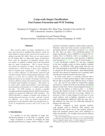
Apparently, the training of the binary classifiers can bedone independently. However, in contrast to the casewhere a single machine is used to train all classifiers andthe major bottleneck is on computation, using a largenumber of machines for training will suffer from file I/Obottleneck since one of our training datasets is as large as1.37 terabyte. If the file I/O bandwith is 20MB/second,simply loading/copying the dataset would take 19 hours.Therefore, we hope to load data as less times as possiblewhile not incurring the computation bottleneck.Our strategy here is to do memory sharing on each multicore machine. Each machine launches several programsto train different subset of the 1000 binary classifiers, andthe programs are synchronized to train on the same chunk oftraining data. The training data is shared by all the programson a machine through careful memory sharing. Therefore,the multiple programs only need to load data once (foreach epoch). Such memory sharing scheme significantlyreduces file loading traffic and speeds up SVM trainingdramatically.70Top 5 hit rate (%)65605550SGDAveraging SGD4540123Epochs45Figure 3. The convergence comparison between ASGD andregular SGD.Histogram of top 5 accuracy1401205. Results1005.1. The performance of ASGD method for SVMtraining8060As aforementioned, the major challenge of the largescale ImageNet classification is on training SVMs withterabytes of training data and as many as 1000 categories.This paper proposes a parallel ASGD method that is aimedto have fast convergence and parallel computation. Fig. 3shows the convergence comparison between the ASGDmethod and the regular SGD method. Both methods wereperformed on the dataset 5 in Table 1 – it is about 1 terabytein total. We see that the ASGD method converged very fast.It reached fairly good solution after 5 iterations. In contrast,SGD (without averaging) converges much more slowly. Itwould take tens of iterations to reach a similarly goodsolution. For this specific dataset, each epoch took about 20hours on three 8-core machines (only 6 programs runningin parallel on each machine due to some limitations).Therefore, ASGD took about 4 days to finish SVM trainingwhile the regular SGD would have taken weeks if notmonths.4020000.20.40.6Accuracy0.81Figure 4. The histogram of the top 5 hit rate of the 1000 classes inImageNet dataset.Indeed, we see a huge improvement in performance fromthe baseline that was reported recently [6], which achievedabout 20% in classification rate. Fig. 4 shows the histogramof the top 5 hit rate on 1000 classes. We see that the top 5 hitrate is mostly concentrated in the range of 60 90% whileit is over 90% for some classes but below 30% for someother classes. The easy classes include odometer, monarchbutterfly, cliff dwelling, lunar crater, bonsai, trolleybus,geyser, snowplow, etc; the difficult classes include Chinatree, logwood tree, shingle oak, red beech, cap opener,Kentucky coffee tree, teak, alder tree, iron tree, grass pink,etc. The detailed top 5 hit rate for each of the 1000 classesis illustrated in Fig. 5.5.2. ImageNet classification resultsWith the proposed ASGD method and 12 eight-coremachines, we were able to train 1000-class SVM classifiersfor all those 6 feature sets listed in Table 1 within oneweek. Classification on each feature set outputs a set ofSVM sores, and we combined them linearly to yield finalprediction.As a result, our classification system achieved 52.9%in classification accuracy and 71.8% in top 5 hit rate.6. DiscussionWe have shown how to train an image classificationsystem on the large-scale ImageNet dataset (1.2 million images) with many classes (1000 classes). We achieved state1694

of-the-art performance on the ImageNet dataset: 52.9%in classification accuracy and 71.9% in top 5 hit rate.The key factors in our system are fast feature extractionand SVM training. We developed a parallel averagingstochastic gradient descent (ASGD) algorithm for SVMtraining, which is able to handle terabytes of data and 1000classes.In this paper, we observed very fast convergence fromthe ASGD algorithm. But we are still not able toquantitatively connect the superior empirical performancewith existing theoretical analysis, most of which focuses onanalyzing the asymptotic convergence property of ASGD.We will study how many training data samples wouldbe needed for ASGD to enter its asymptotic convergenceregime. Work in [23] has done some very interesting analysis in this regard. Meanwhile, we plan to systematicallycompare the ASGD method with other SGD methods (suchas Pegasos [20]) for large-scale image classification.References[1] http://yann.lecun.com/exdb/mnist/.[2] E. Chang, K. Zhu, H. Wang, H. Bai, J. Li, Z. Qiu, and H. Cui.Psvm: Parallelizing support vector machines on distributedcomputers. Advances in Neural Information ProcessingSystems, 20:16, 2007.[3] C. Chu, S. Kim, Y. Lin, Y. Yu, G. Bradski, A. Ng, andK. Olukotun. Map-reduce for machine learning on multicore.In Advances in Neural Information Processing Systems 19:Proceedings of the 2006 Conference, page 281. The MITPress, 2007.[4] C. Cortes and V. Vapnik. Support-vector networks. MachineLearning, 20:273–297, 1995.[5] N. Dalal and B. Triggs. Histograms of oriented gradients forhuman detection. In CVPR, 2005.[6] J. Deng, A. Berg, K. Li, and L. Fei-Fei. What doesclassifying more than 10,000 image categories tell us?ECCV, 2010.[7] M. Everingham, L. Van Gool, C. K. I. Williams, J. Winn,and A. Zisserman. The PASCAL Visual Object ClassesChallenge 2010 (VOC2010) Results. 0/workshop/index.html.[8] R.-E. Fan, K.-W. Chang, C.-J. Hsieh, X.-R. Wang, and C.-J.Lin. Liblinear: A library for large linear classification. J.Mach. Learn. Res., 9, June 2008.[9] L. Fei-Fei, R. Fergus, and P. Peron. Learning generativevisual models from few training examples: an incrementalbayesian approach tested on 101 object categories. In IEEE.CVPR 2004, Workshop on Generative-Model Based Vision,2004.[10] R. Fergus, P. Perona, and A. Zisserman. Object classrecognition by unsupervised scale-invariant learning. InIEEE Conf. on Computer Vision and Pattern Recognition,volume 2, pages 264–271, Wisconsin, WI, June16 - 22 2003.[11] G. Griffin, A. Holub, and P. Perona. Caltech-256 objectcategory dataset. Technical Report 7694, California Instituteof Technology, 2007.1695[12] T. Joachims. Making large-scale svm learning practical.LS8-Report, 24, Universitt Dortmund, LS VIII-Report,1998.[13] T. Joachims. Training linear svms in linear time. In Proceedings of the ACM Conference on Knowledge Discoveryand Data Mining, 2006.[14] S. Lazebnik, C. Achmid, and J. Ponce. Beyond bags offeatures: Spatial pyramid matching for recognizing naturalscene categories. In IEEE Conf. on Computer Vision andPattern Recognition, volume 2, pages 2169–2178, New YorkCity, June17 - 22 2006.[15] Y. LeCun, L. Bottou, Y. Bengio, and P. Haffner. Gradientbased learning applied to document recognition. Proceedings of the IEEE, 86:2278–2324, 1998.[16] D. G. Lowe. Distinctive image features from scale invariantkeypoints. Int’l Journal of Computer Vision, 60(2):91–110,2004.[17] T. Ojala, M. Pietikainen, and D. Harwood. A comparativestudy of texture measures with classification based on featuredistributions. Pattern Recognition, 29:51–59, 1996.[18] B. T. Polyak and A. B. Juditsky. Acceleration of stochasticapproximation by averaging. SIAM J. Control Optim, 30,July 1992.[19] B. C. Russell, A. Torralba, K. P. Murphy, and W. T.Freeman. Labelme: a database and web-based tool for imageannotation. International Journal of Computer Vision, 77(13):157–173, 2008.[20] S. Shalev-Shwartz, Y. Singer, and N. Srebro. Pegasos: Primal estimated sub-gradient solver for svm. In Proceedingsof the 24th international conference on Machine learning,ICML ’07, 2007.[21] T. White. Hadoop: The Definitive Guide. O’Reilly Media,Inc, 2010.[22] S. Y. X. Wang, T. X. Han. An hog-lbp human detector withpartial occlusion handling. In ICCV, 2009.[23] W. Xu. Towards optimal one pass large scale learningwith averaged stochastic gradient descent. Technical Report2009-L102, NEC Labs America.[24] J. Yang, K. Yu, Y.

NEC Laboratories America, Cupertino, CA 95014 Liangliang Cao and Thomas Huang Beckman Institute, University of Illinois at Urbana-Champaign, IL 61801 Abstract Most research efforts on image classification so far have been focused on medium-scale datasets, which are often defined