Transcription
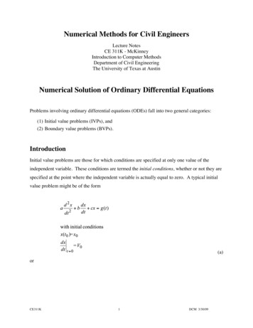
Numerical Methods for Civil EngineersLecture NotesCE 311K - McKinneyIntroduction to Computer MethodsDepartment of Civil EngineeringThe University of Texas at AustinNumerical Solution of Ordinary Differential EquationsProblems involving ordinary differential equations (ODEs) fall into two general categories:(1) Initial value problems (IVPs), and(2) Boundary value problems (BVPs).IntroductionInitial value problems are those for which conditions are specified at only one value of theindependent variable. These conditions are termed the initial conditions, whether or not they arespecified at the point where the independent variable is actually equal to zero. A typical initialvalue problem might be of the form(a)orCE311K1DCM 3/30/09
(b)The variable which is being differentiated is called the dependent variable, x in this case, and thevariable with respect to which the dependent variable is differentiated is called the independentvariable, t in this case. When the problem involves one independent variable, the equation iscalled an ordinary differential equation. Differential equations are classified as to the highestorder derivative appearing in them. In the case of Equation (a), the differential equation is ofsecond order; Equation (b) is of first order. Equation (a) could describe the forced response of asimple harmonic oscillator with time. Since Equation (a) is a second-order differential equation,two conditions have been specified at t 0.Boundary value problems are those for which conditions are specified at two values of theindependent variable. A typical boundary value problem might be of the formThis problem could describe the steady-state temperature distribution in a rod of length L withtemperatureatandat. These are called the boundaryconditions.CE311K2DCM 3/30/09
Initial Value ProblemsAny initial value problem can be represented by a set of one or more coupled first-order ordinarydifferential equations, each with an initial condition. For example, Equation (a) can be restatedby making the substitutionThe differential equation is then written asWith some rearrangement, the problem can now be written aswith initial conditions (one for each equation in the set):Since any initial value problem can be reduced to a set of first-order ordinary differentialequations, we shall concentrate on numerical methods for the solution of first-order differentialequations Thus, we consider an initial value problem of the formCE311K3DCM 3/30/09
. The next step isSuppose that we know the solution to this equation over the intervalto advance the solution toby extrapolation. We will consider techniques of theRunge-Kutta type, where the desired solutionis obtained in terms of,, andevaluated for various estimated values of x between ti and ti 1. The first such techniqueis Euler’s method and is discussed in the next section.Figure 3. Initial value problem intermediate solution. Solution is known to ti solution is desiredat ti 1.Euler’s MethodConsider the first-order initial value problemCE311K4DCM 3/30/09
One solution method is to replace the derivativeby a simple forward finite differenceapproximationSolving foryieldsGiven an initial condition,, it is possible to proceed forward in time from t0, to obtaina value of x at each new value of t. The slope at the beginning of an interval,, is takenas an approximation of the average slope over the whole interval as shown in Figure 2. The newvalue of x, at, is predicted using the slope at the old point, xi, to extrapolate linearly over thestep size t.CE311K5DCM 3/30/09
Figure 4. Illustration of Euler’s method.Example: Use Euler’s method to find a numerical approximation for x(t) wherefrom t 0 to t 4 using a step size of t 0.5.By simple integration, the exact solution to this equation isThe Euler formula for this equation isCE311K6DCM 3/30/09
Starting at t 0 (i 0) and using t 0.5, we find x at t 0.5The exact solution at this point isNext, we can advance the solution from t 0.5 (i 1) and find x at t 1.0, using the value wejust found as an initial conditionThe exact solution at this point isThe calculations for several steps are plotted in Figure 5. A C program for computing the answerto this problem using Euler’s method is presented in Figure 6. The error in the calculations isillustrated in Figure 7. The error in these calculations stems from two factors: (1) the use offinite precision arithmetic in the computer (roundoff error); and (2) the truncation of the Taylorseries in the finite difference approximation of the first derivative in Euler’s method (truncationerror).CE311K7DCM 3/30/09
Table. Results of Euler Method 0.501.001.502.002.503.003.504.00dt 000.500.710.890.750.400.280.421.33Figure 5. Euler method exampleCE311K8DCM 3/30/09
Figure 6. Error in Euler method example.Runge Kutta FormulasAmong the most widely used formulas for numerically solving ordinary differential equationsare the Runge-Kutta techniques. High-order accuracy can be obtained by evaluating the righhand-side function at selected points within the interval rather than at just the end points of theinterval. Consider again the first-order initial value problemCE311K9DCM 3/30/09
In the development of the Runge Kutta formulas, we assume that the estimate of the solution x(t)iswhereThat is, the increment x is a weighted sum of function evaluations at points within the interval. If we cut this estimate off after the first term, we havewhereNow, if we set w1 1, the result is Euler’s method (first-order Runge Kutta)If, instead, we cut the estimate off after the second term, we havewhereCE311K10DCM 3/30/09
Now, if we set w1 w2 and c2 a21 1, the result is the modified Euler’s method (secondorder Runge Kutta)This method is implemented asFigure 7. Modified Euler method.The most widely used Runge-Kutta method is the fourth-order method, where we cut theestimate off after the fourth termCE311K11DCM 3/30/09
whereandw1 w4 1/6,w2 w3 1/3 andc2 c3 a21 a32 1/2, c4 1, anda31 a41 a42 0The computational formula for the Fourth-order Runge-Kutta method iswhereExample:Analytical solution:CE311K12DCM 3/30/09
Euler method:Modified Euler (second-order Runge-Kutta) method:Fourth-order Runge-Kutta method:whereCE311K13DCM 3/30/09
Figure 8. Analytical solution versus Euler method approximation for two levels of discretization( t 0.5 and t 1.0).Table 1. Analytical solution versus Euler method approximation for three levels ofdiscretization ( t 0.5, t 1.0, and t 2.0).tanalyticalEuler ( t 1.0)Euler ( t 2.0)Euler ( t E 06Table 2. Modified Euler method (2-nd order Runge Kutta) approximation ( t 0.5).CE311K14DCM 3/30/09
tModified Eulerxi* ( t .092Table 3. Fourth order Runge Kutta approximation ( t .009-0.008-0.007-0.006-0.006-0.005-0.005-0.004xi 50.091DCM 3/30/09
Figure 9. Comparison of analytical, Euler (1-st order RK), modified Euler (2-nd order RK), and4-th order Runge Kutta approximation ( t 0.5).Table 4. Comparison of analytical, Euler (1-st order RK), modified Euler (2-nd order RK), and4-th order Runge Kutta approximation ( t 0.1050.100Mod. h Order 820.1670.1540.1430.1330.1250.1180.1110.1050.100DCM 3/30/09
dary Value ProblemsRecall that boundary value problems are those for which conditions are specified at two valuesof the independent variable. A typical boundary value problem might be of the formwith boundary conditionsTwo methods are commonly used to solve boundary value problems: (1) the shooting method,and (2) finite-difference methods.Section under constructionExample: Flow in a leaky confined aquiferConsider the steady flow from left to right in the semi-confined aquifer shown in Figure 2. Theaquitard is leaky. Determine the head in the aquifer.Figure. Flow in a leaky-confined aquifer.CE311K17DCM 3/30/09
The governing equation for flow in the aquifer can be written as K h K (h h) 0b 0If the aquifer is considered to be homogeneous and isotropic, we can write this equation as 2h h0 h 0 2where 2 bKb’/K’. Now for one-dimensional flow, we haved 2h h h0dx 22a second-order ordinary differential eqaution with constant coefficients which has the solution(hA h0 )sinh(h(x) h0 L xx) (hB h0 )sinh( ) Lsinh( ) Consider the values L 1000 m, HA 100 m, Hb 80 m, K 20 m/day (clean sand), B 50 m,B’ 2 m, K’ 0.10 m/day (silt), n 0.35. The head distributions for the values of h0 are shownin Table 1 and plotted in Figure 3.Figure. Semi-confined aquifer head values for various overlying aquifer head levels.CE311K18DCM 3/30/09
Table. Semi-confined aquifer head values for various overlying aquifer head levels.Xh0 110h0 105h0 100h0 95h0 900.00100.00100.00100.00 100.00 1000.0080.0080.0080.0080.0080.00Systems of Ordinary Differential EquationsConsider the system of ordinary differential equationsExample: Find a solution to the following system of two ODE’s using fourth-order RungeKutta on the interval 0 x 2, x 0.5CE311K19DCM 3/30/09
with initial conditionsThe formulas for fourth-order Runge-Kutta method arewhereandFor the example problem:1) Compute some K values:CE311K20DCM 3/30/09
2) Compute some intermediate y valuesand some K values3) Compute some more intermediate y valuesand some K values4) Compute some more intermediate y valuesand some K valuesCE311K21DCM 3/30/09
5) Now, compute the next y valuesRepeat steps (1) - (5) for i 1,2,3,4.Example: Predator - Prey models (Ricklefs, p. 536)In an ecosystem, the size (number) of the prey population is H and the rate of growth of the preypopulation () is comprised of two components:1) Unrestricted reproductive rate (growth rate) of prey population g1H, where g1 is the growthrate of an individual in the population.2) Removal of prey from the population by predators (death rate). This is assumed to beproportional to the product of the prey and predator population sizes (PH, this term isproportional to the probability of an encounter between predator and prey) times a coefficientof predation d1.Thus, the overall increase in the size of the prey population is given byThe growth rate of the predator population is proportional to the number of prey that the predatorsucceeds in capturing (d1PH) minus the death rate (d2) times the number of predators (P)CE311K22DCM 3/30/09
where g2 ad1, and a is the efficiency with which predators convert food (prey) into offspring.When the predator and prey populations are in equilibriumwhere P* is the greatest number of predators that the prey population can sustain, andwhere H* is the minimum level of prey population required to sustain the predators.Example: (Chapra and Canale, prob. 22.20)If P(0) 5, H(0) 20, g1 1, g2 0.02, d1 0.1, d2 0.5, compute P(t) and H(t) from t 0 to 10using the fourth-order Runge-Kutta technique and t 0.5.Reactor Mass BalanceConsider the conservation of mass in a fully mixed reactor vessel as shown in the followingFigure.CE311K23DCM 3/30/09
Figure 10. Conceptual diagram of a reactor vessel with 1 inlet and 1 outlet.Conservation of mass is a mass balance accounting of the material passing in or out of thereactor vessel, whereRate of Mass Input - Rate of Mass Output Change in Mass Storage (Accumulation)At steady-state, we haveChange in Mass Storage (Accumulation) 0orRate of Mass Input Rate of Mass OutputHowever, if steady-state conditions do not exist in the system, then we must consider the timerate of accumulation of the substance in the reactorAccumulation whereM is the mass of chemical in the reactor, andCE311K24DCM 3/30/09
V is the (constant) volume of the reactorSo thatFor example, if the vessel has is a single inlet and a single outlet, thenIf c c0 @ t 0, then the solution of this ODE isIf cIN 50 mg/m3, Q 5 m3/min, V 100 m3, and c0 10 mg/m3, we haveEuler's method can be used to approximate the solution to the ODE.orNow, plugging in the numerical values, we haveCE311K25DCM 3/30/09
Question: What would the formulas for the modified Euler method look like?5045Conc.(mg/m )Figure 11. Comparison of analytical solution and Euler approximation.System of Coupled ReactorsConsider the 5 interconnected reactors shown in the Figure. We can write 5 simultaneous massbalance equations, one for each reactor,CE311K26DCM 3/30/09
Now we must solve a system of ODE's instead of a single ODE. We can still apply the Eulermethod to this system.Which may be written in a matrix-vector notation asCE311K27DCM 3/30/09
c5Q54Q15Q01, c01c1Q55Q25Q12c2Q24c4Q44Q 23Q13Q34c3Q03, c03Figure 12. System of 5 interconnected reactors.Exercises1. Solve the following initial value problem analytically over the interval from x 0 to 2:where y(0) 1. Plot the solution.2. Use Euler’s method with h 0.5 and 0.25 to solve Problem 1. Plot the results on the samegraph to visually compare the accuracy of the two step sizes.3. Use the Modified Euler method with h 0.5 and 0.25 to solve the following initial valueproblem analytically over the interval from x 0 to 2:where y(0) 1. Plot the solution.4. Use the 4-th Order Runge – Kutta method with h 0.25 to solveCE311K28DCM 3/30/09
where y(0) 1. Plot the solution.5. (a) What are the advantages and disadvantages of using the Euler method to solve anOrdinary Differential Equation rather than using a 4-th Order Runge-Kutta method? (b) Solvethe following Ordinary Differential Equation using the Euler method from t 0.0 to 1.0 with t 0.2.6. Use the Euler method and a step size of t 0.25, solve the initial value problem on theinterval t [0, 1]where x(0) 1.7. Population growth of any species is frequently modeled by an ordinary differential equationof the formdNdt aN bN2N(0) N0where N is the population size, aN represents the birth rate, and bN2 represents the death rate dueto all causes, such as disease, competition for food supplies, and so on. If N0 100,000, a 0.1,and b 8x10⁻⁷, calculate N(t) for t 0 to 20 using t 1.8. The population of two species competing for the same food supply can be modeled by thepair of ordinary differential equationsdN1 dtN1(A1 B1N1 C1N2 )N1(0) dN2dt N2 (A2 B2N2 C2 N1)N2 (0) CE311KN1,029N2,0DCM 3/30/09
where AN is the birth rate, and BN2 represents the death rate due to disease, and CN1N2 modelsthe death rate due to competition for the food supply. If N1,0(0) N2,0(0) 100,000, A1 0.1,B1 8x10⁻⁷, C1 1x10⁻⁶, A2 0.1, B2 8x10⁻⁷, C2 1x10⁻⁶, calculate N1,0(t), and N2,0(t) for t 0 to 10 years using t 1.9. Solve the following pair of ODE's by the Euler method from t 0.0 to 1.0, with t 0.2:10. The following equation is used to describe the conservation of mass for a reservoirdSdt I(t) Q(H ) (1)where S is the volume of water in storage in the reservoir, I(t) is the inflow into the reservoir as afunction of time t, and Q(H) is the outflow from the reservoir, which is determined by theelevation H of water in the reservoir. The change in volume S of the water in the reservoir, dueto a change in the water depth dH , is expressed asdS AdHwhere A is the area of the reservoir (assumed constant in this problem) and H is the elevation ofthe water surface. Equation (1) can then be written asdHdt 1[I(t) Q(H)]A(2)Develop the equations necessary to solve Equation (2) using the fourth-order Runge Kuttamethod (just set up the equations!). Assume that the function I(t) is known andCE311K30DCM 3/30/09
Q(H ) H where and are constantsdH f (H, t) dtH(t 0 ) H01[I(t) H ]A11. The following equation describes the steady-state diffusion of a dissolved substance into aquiescent fluid body in which a first-order reaction occurs:Dd 2cdx 2- Kc 0(1)with boundary conditions:c(0) 0, c(1) C1where c(x) (M/L3) is the concentration of the dissolved substance, D (L/T2) is the diffusioncoefficient, K (1/T) is the reaction rate, and C1 (M/L3) is a specified concentration on the rightboundary of the domain.(a) Write a finite-difference approximation of Equation (1)(b) Using 3 evenly spaced nodes with node spacing x 0.5, write the finite difference equationthat you developed in part (a) for each node at which the concentration is unknown in thesystem.(c) Solve for the unknown concentration using the numerical values for the coefficients:D 0.01 cm2/s, K 0.1 s-1, and C1 1.0 g/cm3.CE311K31DCM 3/30/09
12. Water quality models can be used to predict the concentration of various constituents inreceiving waters (streams, lakes, and rivers). Many of these models are extensions of the twosimple equations proposed by Streeter and Phelps (1925)1 for predicting the biochemical oxygendemand (BOD) of various biodegradable constituents, and the resulting dissolved oxygen (DO)concentration in rivers. The BOD concentration (B) and the dissolved oxygen deficitconcentration (D) (i.e., the difference between the water's saturated dissolved oxygenconcentration and the actual concentration--see Figure below) in a river are functions ofsimultaneous reactions which can be described by the equations:dB Kd BdtdD Kd B Ka Ddt(1)where Kd is the deoxygenation rate constant (T-1), Ka is the reaeration rate constant (T-1), and t[T] is the time of flow along a section of river. The solution of these equations for a single wastedischarge at the beginning of a river section results in the dissolved oxygen sag curve shown inthe following Figure.1Streeter, H.W., and E.P. Phelps, A study of the pollution and natural purification of the Ohio River, U.S. PublicHealth Service, Publication Health Bulletin 146, Feb. 1925.CE311K32DCM 3/30/09
DissolvedoxygenconcentrationSaturated dissolvedoxygen concentrationInitial DeficitD0Deficit DiDissolved oxygenconcentration curveXiDistance downstream XX0Figure. Dissolved oxygen "sag" curve resulting from single point discharge of BOD and initialoxygen deficit concentration at X 0.Initial BODdischarge, B0Initial DOdeficit, D0D(X)River sectionXFigure. River section showing initial DO deficit and BOD discharge location.(a) Develop the equations for applying Euler's method to solve the Streeter-Phelps equations forboth BOD, B, and dissolved oxygen deficit, D.(b) Solve for the BOD, B, and dissolved oxygen deficit, D, in the river using the Euler methodequations that you developed in part (a) using the following data:CE311K33DCM 3/30/09
Kd 0.3 day-1 deoxygenation rate constantKa 0.4 day-1 reaeration rate constantDsat 8 mg/L Saturated dissolved oxygen concentrationD0 1.0 mg/L Initial dissolved oxygen deficitB0 15 mg/L Initial BOD concentration at the beginning of the river section t 3/4 dayTake 3 steps of the method.13. Using the modified Euler method (second-order Runge Kutta method), take two steps of t 0.1 for the following initial value problem4tdy ty,ydty(0) 3a) 13 pts. Solve the following Ordinary Differential Equation using the Euler method from t 0.0 to 1.0 with t 0.2.14. Euler method for systems In the classic Lokta-Volterra equation of predator - preymodeling, the overall increase in the size of a prey population is given bywhere H is the size of the prey population, P is the size of the predator population, g2 is thegrowth rate of the prey population, and the death rate is d2. The predator population is governedby the equationCE311K34DCM 3/30/09
where g2 is the growth rate of the predator population, and the death rate is d2.(a) Show the formulas for the Euler method of solving these 2 ordinary differential equations(Don’t plug in any numbers yet, just show the formulas.)(b) Consider the initial conditionsP(0) 5, H(0) 20and the numerical valuesg1 1, g2 0.02,d1 0.1, d2 0.5Compute P(t) and H(t) from t 0 - 1.5 using the Euler method and t 0.5.(b.1) Show the calculation for the first time step (from 0 to 0.5)(b.2) Show the calculation for the second time step (from 0.5 to 1)(b.3) Show the calculation for the third time step (from 1 to 1.5)( c) Explain the solution of these equations in terms of the sizes and behavior of the populations.15. Leaky acres. Consider the steady flow from left to right in the leaky aquifer shown in theFigure. The aquitard is leaky. If there is no leakage up from below and flow in the aquitard isvertical, and we have another aquifer above the aquitard where the head is h0 , for onedimensional flow indicated in the figure, we haveCE311K35DCM 3/30/09
where 2 bKb’/K’ is called the leakage factor, K is the hydraulic conductivity and b is theaquifer thickness, h is the average head at a point in the aquifer, , and K’ and b’ are theconductivity and thickness, respectively, of the confining layer (aquitard).Figure. Flow in a leaky-confined aquifer.Consider the values L 1000 m, x 200m, HA 100 m, HB 80 m, K 20 m/day (clean sand),b 50 m, b’ 2 m, K’ 0.10 m/day (silt). The head distributions for values of h0 (head in theoverlying aquifer) are shown in the Table.(a) Apply a second-order accurate finite-difference approximation to the second derivative andwrite out the resulting equation.(b) Write out the finite-difference equation for each node i where the head is unknown, that is,nodes 1 - 4.( c) Show the resulting system of equations, written in matrix-vector form, if you move all theknown values to the right-hand-side of the equation and leave the unknowns on the left.(d) Discuss how you would solve this system of equations using a computer. Draw a simpleflowchart of your method of solution.16. Use Euler’s method to find the solution to the initial value problem:CE311K36DCM 3/30/09
Compare your result atwith the value of the exact solutionat the same point.17. Modified Euler Method. a. Solve the following initial value problem analytically over theinterval x 0 to 1.where y(0) 1.b. Use the Modified Euler method with h 0. 5 to solve the following initial value problem inPart (a) over the interval from x 0 to 1:18. Consider the following initial value problem:(a) Use Euler’s method to solve the initial value problem.(b) Use the Modified-Euler method to solve the initial value problem.(c) Compute the percent relative error from parts (a) and (b) at t 0.5 by comparing to the valueof the exact solutionCE311K37DCM 3/30/09
Numerical Methods for Civil Engineers Lecture Notes CE 311K - McKinney Introduction to Computer Methods Department of Civil Engineering The University of Texas at Austin Numerical Solution of Ordinary Differential Equations Problems involving ordinary differenti

