Transcription
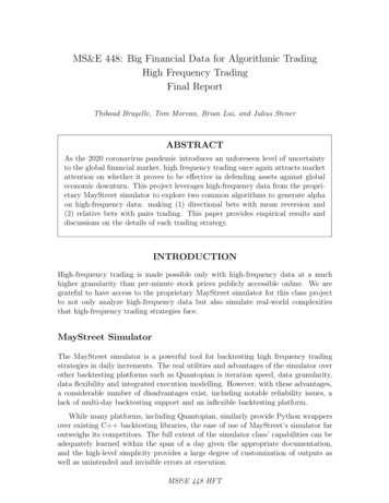
Fundamental Signals for Algorithmic TradingMS&E 448 Final ProjectJames Wong, Yanni Souroutzidis, Max Lai, Evelyn Mei, Ankit SagwalDr. Lisa Borland (supervisor)June 6, 2016AbstractThe project aims at analyzing the impact and making use of fundamental signals to predict the future stock price performance of equities. Welooked at a number of signals - firm’s financial performance metrics andratios (fundamental signals), critical events and public sentiment. Afterdiscussing potential approaches, we decided to start with the Healthcaresector to develop the core algorithm before moving on to other sectors(Technology). The strategy hypothesizes that fundamental and sentiment signals could be good predictors of stock price performance. Theengine is based on machine learning - we trained and optimized a randomforest model to make predictions. The project has given us a good understanding of which factors are important in making predictions. But moreimportantly, through this effort, we were able to develop a framework totest fundamental based algorithms for predictive power. This was criticalsince outperformance in test scenarios is not a sufficient condition for agreat algorithm.1Data CollectionWe started our project focusing on the Healthcare sector. The impetus forthis was because we originally wanted to explore event-driven trading whichwould be done through mining clinical trial data in addition to other datasetsavailable to us. After developing a reasonable model for the Healthcare sector,we extended our work to other sectors such as Technology.The features we explored include: fundamental data, sentiment data, clinicaltrial data, and stock price and volume data. Raw feature data is very skewed andnot predictive by itself. For example in Figure 1 we can see that there is a widerange of values for working capital fundamental values, and the predictabilityof short term returns or long term enterprise value has a high variance. Toresolve this we derived the stock’s feature value normalized with the particularstock’s past feature values (rather than taking the raw feature value) and tookthe z-score to get a cleaner signal.1
Figure 1: Processing raw feature data to obtain cleaner, more predictive signals.1.1Fundamental DataFundamental data is provided by Morningstar which is integrated with Quantopian. There are 13 categories of fundamental data and over 600 total metrics.To select the top fundamentals to use in our final model, we (1) trained randomforest (and other) models on each category of fundamental data, (2) selectedthe top 10 to 15 features from each category by feature importance (feature importance will be described in Section 3.1: Feature Selection), and (3) retrainedthe models using the top features within each category to obtain the overalltop features. The reason to obtain the top features within each category andthen merging was because of a technical limitation to the number of featureswe could train at one time using the scikit-learn library.1.2Sentiment DataThe sentiment data was provided by PsychSignal which derives bullish andbearish scores from Twitter and StockTwits data. Categorization of whether anindividual message is bullish or bearish is determined by PsychSignal’s algorithmand a score is provided as to how bullish or bearish a message is. To obtain aclearer and more consistent signal, we took the 30-day average of the messagescores.1.3Clinical Trial DataThe clinical trial data was provided by Quantopian as a .csv file containingthe phases, outcomes, and indications of each clinical trial update. The datawas too sparse as some companies were missing clinical trial events or did nothave complete coverage, and loading the .csv file required a lot of computationaloverhead which caused the backtester to timeout, so we did not use the data aspart of our model.1.4Stock Price & Volume DataFeatures were also derived from the stock’s price and volume data. Importantfeatures included the 30-day moving average of stock price and volume averagedover the past month, average volatility over the past month, and average returnpercentage over the past month.2
2Machine Learning ModelsThe types of machine learning models we explored include the random forest,extremely random trees, and logistic regression models. The machine learningmodels are used to predict short term returns and long term change in enterprisevalue. For the two tree-based models, we experimented with both regressionand classification models (regression models predict continuous values whereasclassification models predict class or category labels), and for logistic regressionwe experimented only with a classification model.With the tree-based models, we tuned the models by modifying the depth ofeach tree, the total number of trees in the model, and the number of variables tochoose from at each node split. Both of the tree-based models we experimentedwith are ensemble learning methods consisting of multiple decision trees. Theindividual subtrees of the random forest model are generated by optimizing forinformation gain where each node split is determined by the split resulting inthe largest reduction of entropy.Entropy(S) cX pi log2 pii 1XGain(S, A) Entropy(S) v V alues(A) Sv Entropy(Sv ) S Figure 2: Entropy and information gain in a decision tree.This is in contrast to the training of the extremely random trees model whereeach node is split randomly [2]. The final prediction of the ensemble is the modeor mean of the individual decision trees depending on whether we are modelingclassification or regression, respectively.In machine learning, there is a tradeoff between bias and variance. Biascauses the algorithm to miss relevant information embedded in the features(underfitting), and variance causes the algorithm to overcompensate for smallintricacies or noise of the training data (overfitting). Decision trees typicallysuffer from overfitting (low bias, high variance) especially when the depth sizeor number of nodes is high. However randomness of the random forest, where thesubset of features used to train each subtree is random, and extremely randomtrees, where the node splits are also random, help the overall ensemble achievelower variance at the cost of slightly higher bias.The machine learning models were used to predict the following: (1) longterm changes in enterprise value (over six months) using signals from fundamental data, and (2) short term returns (over one month) using signals fromthe long term model and sentiment, clinical trial, price, and volume data. Thenext section further describes how we collected our training data. From ourwork, we found the random forest to perform the best so we spent the mosttime on random forests throughout our project. Extremely random trees weresignificantly faster to train and was comparable to the random forest but hadhigher variance. The logistic regression model did not perform well relative tothe tree-based models even if we compared amongst classification models.3
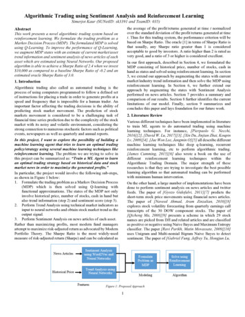
2.1Training Data CollectionCollecting training data for the classification and regression models was similar.For the short and long term models, we used data from the past few years andcomputed the percentage change in stock price (returns) over one month andpercentage change in enterprise value over six month time intervals, respectively.For regression models, the raw percentage change was used as the label, and forclassification models we assigned labels of -1, 0, and 1 for when the stock priceor enterprise value decreased by over 3%, stayed within 3%, and increased byover 3%; respectively; within the time interval. We empirically found the 3%threshold to be the most effective. All the training data was collected out ofsample and used to predict future values in both the backtester and researchmode. We also experimented with increasing the amount of training data byincreasing how far back we collected training data from. For sentiment data, wewere constrained because data is only available starting in 2010. The clinicaltrial data coverage was from 2007 to 2015, and we did did not end up using itdue to its sparseness.3Residual Analysis and ForecastVarious approaches were used to assess each model before going into backtestruns and to get an understanding of the model.3.1Feature SelectionTo understand the predictability of each feature, we calculated feature importance within the ensemble tree-based methods. We trained models and analyzedthe feature importance which is a measure of the information gain given by eachfeature [3].Imp(Xm ) 1 XNTTXp(t) i(st , t)t T :v(st ) XmFigure 3: Feature importance calculation.The five most important fundamental features as shown below in Figure 4were book value per share, market cap, book value yield, cash flow yield, andsales yield. While the feature importance ranking varied from sector to sector,these features generally made it to the top across most sectors.Figure 4: Feature importances for fundamentals on the Healthcare sector.4
3.2Model AssessmentTo assess the model before going into backtests, we analyzed the (1) directionality accuracy of the model (e.g. if the model prediction and the actual outcome align in positive, negative, or neutral direction), (2) correlation betweenpredicted and actual returns or change in enterprise value (R-squared), and (3)overall distribution of predicted vs. actual returns or change in enterprise value.These metrics are illustrated in Figures 5-7 below.Figure 5: Directionality accuracy of the enterprise value long term model overtime. In general, the model is directionally accurate for most months.Figure 6: Correlation between predicted vs. actual short term returns. Thecorrelation here is quite low with a R-squared value of 0.009.Figure 7: Overall distributions of predicted vs. actual change in enterprisevalue.5
When tuning the machine learning models, we also leveraged the three metrics to find the best training parameters of the random forest. As we increasedthe number of trees and the tree depth, we found the correlation between predicted and actual enterprise value to increase and the overall distributions ofpredicted and actual enterprise value to also converge, as shown in Figures 8and 9.Figure 8: Healthcare sector results for random forest models using 500 trees ofdepth 15 and 1000 tress of depth 15.Figure 9: Healthcare sector results for random forest models using 1000 treesof depth 20 and 2000 tress of depth 25.Extending these models into the Technology sector, we obtained similarresults as those of the Healthcare sector in Figure 10. The overall feature importances were also similar to those for the Healthcare sector.Figure 10: Technology sector results for a random forest model using 2000 treesof depth 25.6
4Core Model & Trade ExecutionFigure 11: Flow diagram of the trading algorithmWe considered three distinct elements when executing our trades: signalgeneration, risk management and portfolio optimization. The algorithm implements these elements as follows (also illustrated in Figure 11):4.1Signal GenerationWe use a machine learning model to make predictions. The input to the machinelearning model is a set of fundamental and sentiment signals, and the returngenerated by a stock over one month periods (the time is flexible, as you willsee in the multiple approaches we tried). We then train our machine learning topredict monthly returns in the future. At the start of every month, our modeloutputs a prediction of monthly returns expected in each stock, based on thesignals observed in them. This drives the trade decisions - higher the predictionfrom the model, more we want to buy that particular stock.4.2Portfolio ConstructionWe consider the top 15 recommendations from the model and allocate capitalequally between the stocks. In subsequent trades, if a particular stock is alreadyin the portfolio, then we relax our criteria of top 15 for that stock, and include itas long as it falls within the top quartile of buy recommendations. The buyingdecision is also based on the liquidity available in the stock. Whenever we seesmall trading volumes in comparison to the amount we want to buy, we divideour execution over multiple days to avoid slippages (or failed execution) in theQuantopian backtest environment.4.3Risk managementIf a particular stock in the portfolio performs poorly during the month (whenthe model is not making predictions), we trigger our stop loss and exit that7
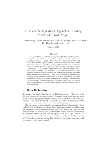
particular position. Currently, the two triggers in place are - Loss of more than10% in value in a week, or loss of more than 10% since taking the position. Theintuition here is to avoid getting into traps where a stock falls significantly dueto external reasons and we lose a lot of value before our model gets to the nextmonth’s prediction.4.4Future ImprovementsIf we were to develop this model further in the coming months, some importantareas to improve on would be (also refer Section 7: Future work) - Dynamicallydecide number of positions to hold each month, and allocate capital based onthe strength of the signal output from the prediction model. Dynamic stop lossdetermination, which the model can decide based on the sector, volatility andmarket capitalization of the stock. Manage portfolio risk through covarianceanalysis of existing positions. This could also serve as one of the features insidethe prediction model. The feature would depend on the existing portfolio, andwould aim to minimize risk in the portfolio. Index shorting can also be employedto hedge against risk.5Strategy PerformanceThe performance of our short-term monthly updating algorithm is shown below.We tested our algorithm by backtesting on the Pharmaceutical sector in theQuantopian platform and taking different combinations of the datasets available(twitter data, clinical trials data and fundamentals data). Although the longterm enterprise model is more rigorous, we are unable to implement this onthe Quantopian backtest framework since it times out before the tests can becompleted. Hence, we will just show performance results of the short-termmonthly algorithm as shown in Figure 13. The 4 different datasets combinationsthat we tested on our algorithm are: Twitter data only Fundamentals data only Twitter data and fundamentals data only Twitter data and clinical trials data and fundamentalsFigure 12: Summary of the performance of different dataset combinations.We see that if we just use the Twitter data, we do not achieve strong predictions, as we obtain a negative alpha and low sharpe ratio combined with a8
Figure 13: Quantopian backtests of the different dataset combinations.relatively high beta. Using just the fundamentals data, we obtain a much higheralpha and sharpe ratio with the same beta.We investigated and found that combining more datasets in our algorithmdoes not improve the predictions generated. We tested different combinationsof the dataset, two of which are shown in the bottom of Figure . We see fromthe statistics in Figure 12 that adding additional datasets to the fundamentalsdata actually decreases alpha and sharpe without improving beta and volatility.We believe that this is because there is too much noise in the Twitter andclinical trials dataset, which results in the generation of a weaker predictivemodel (overfitting to the nuasances of the training data and noise).From our results, it seems that only using the fundamentals data generatesthe best predictive model. It has a strong sharpe ratio of 1.5. However, itshould be noted that past performance is not indicative of future results - allthat glitters is not gold [5]. From the backtest, we see that the model essentiallyperformed the same as the S&P 500 for prolonged periods of time and theoutperformance was due to two stretches of spectacular returns. It is not knownif this can be repeated in a future time period.To see if this performance can be generalized to different sectors, we appliedthe fundamentals data only model onto the Technology sector. The backtestis shown in Figure 14. We can see that the performance of the model remainssteady. This supports the notion that we have built a robust model that can begeneralized to other sectors.Figure 14: Fundamental data only backtest on Technology sector.9
6SummaryUsing publicly available data, we have built an algorithm that generates mildlyaccurate predictions on the future stock price of companies. While we do notbelieve that substantial profits can be generated from the algorithm, we trustthat it can be added to an investor’s arsenal of indicators to generate betterreturns. It makes intuitive sense that any model based on publicly availablefundamental signals to predict stock price performance has to be reasonablycomplicated and many easy predicted outcomes would already have been exploited by quantitative hedge funds to make returns. Most of these potentialprofits would then be arbitraged away by an efficient market.If we were to undertake this project once again, we would have proceededslightly differently to save a considerate amount of time. We would have focused on implementing the algorithms on the research environment instead ofthe backtest environment, which often had technical issues. We would have alsospent less time on trying to build a model based on the clinical trials dataset,which was ultimately unsuccessful due to the technical capacity of the Quantopian backtest environment.Overall, we are pleased to better understand the space of fundamental basedalgorithm trading and to have developed a mechanism to check future algorithmsfor robustness, rather than depending on only backtest runs. In the future, wewould like to explore further and hope to develop more predictive power in ouralgorithms.To deploy our model and system into the real world, Quantopian allows foralgorithms to go live with a linked Robinhood or Interactive Brokers account.After some adjustments, we would be interested in deploying our system into aQuantopian contest or for live trading.7Future WorkWhile we have accomplished much during the 10-week project, we believe thatthere is still ample room for further exploration in the journey of developing aconsistent high sharpe ratio algorithm. We have identified three areas that webelieve could be further explored given a longer project timeframe.One improvement that can be made to our project is to perform better datapre-processing. Specifically, we believe that there is substantial room for improvement in the way we treat gaps in the dataset. Currently, we have replacedall gaps with -2, an arbitrary number. This does not really make sense for somefeatures, such as market capitalization, as they cannot realize a negative number. Additionally, replacing substantially different rows that have the same gapwith the same constant can seriously distort the regression results. To improvewe can use machine learning algorithms such as k-nearest-neighbors and localregression to improve our prediction of these values based on the values of therest of the features. This is not a simple problem, as we also need to figure outhow to account for the fact that different rows have different amounts of datamissing on different features.Another improvement that can be made is to look at additional machinelearning algorithms. During the design process, we looked at several models,including linear regression, interaction terms and random forests. From the test10
results, we see that of all the machine learning techniques we have implementeda tuned random forest predictor performs the best. However, there are plenty ofother machine learning algorithms that we can try implementing, such as NeuralNetworks and Support Vector Machines. We can also consider building our ownadaptation of a machine learning algorithm using a unique loss function.Given substantially more time, we also believe it would be prudent to buildour own research platform to allow us to obtain substantially greater processingpower for our algorithms. Currently, the Quantopian backtest environmentwill time out after 6 minutes. Additionally, since scripts are run on the internalQuantopian server, both the backtest environment and the research environmentrun (very) slowly with no conceivable method of speeding up. We frequentlypassed this 6 minute time limit and in fact had to abandon using the clinicaltrials dataset because the Quantopian framework took too long to process theinput file. This is a problem, as our tests have shown that our algorithms showslight improvements in predictive ability as the depth of our trees increases.With our own research platform, which we can create by extracting the necessarydata from Quantopian, we are given substantially more freedom to generatemore complex learning algorithms. For example, we can quickly implementthe first two points above by paralleling the computations on our own server(otherwise it could take a substantial amount of time).11
References[1]K. Daniel and S. Titman. “Market Reactions to Tangible and IntangibleInformation”. In: The Journal of Finance (2006).[2]Pierre Geurts, Damien Ernst, and Louis Wehenkel. “Extremely randomizedtrees”. In: (2006).[3]Gilles Louppe et al. “Understanding variable importances in forests of randomized trees”. In: (2013).[4]J. Piotroski. “Value Investing: The Use of Historical Financial StatementInformation to Separate Winners from Losers”. In: Journal of AccountingResearch (2000), pp. , 38, 1–41.[5]Thomas Wiecki et al. “All that Glitters Is Not Gold: Comparing Backtestand Out-of-Sample Performance on a Large Cohort of Trading Algorithms”.In: (2016).12
8Appendix - Valuation MethodologyFundamental analysis and technical analysis are two major schools of practicefor evaluating stocks. Fundamental analysis is a technique that attempts todetermine a security’s intrinsic value by examining underlying factors that affect a company’s actual business and its future prospects. These factors canbe both qualitative and quantitative, concerning macroeconomic, such as theoverall economy and industry conditions, as well as company-specific factors,like financial condition and management. Fundamental analysis helps estimatethe intrinsic value of the firm, which can be used to compare against the security’s current price, based on which, long short positions are taken accordingly(if underpriced, long; if overpriced, short) In general, there are two ways ofconducting fundamental analysis8.1Method 1: Discounted free cash flow modelStock P rice M arket V alue of EquityN umber of Shares OutstandingEnterprise V alue Cash DebtN umber of Shares OutstandingWhere the current enterprise value isV0 F CF1F CFNVNF CF2 . 1 rW ACC(1 rW ACC )2(1 rW ACC )N(1 rW ACC )NAndF CFN F ree Cash F low in Y ear NV0 Current Enterprise V aluerW ACC Discount Rate Determined by W eighted Average Cost of CapitalVN Enterprise V alue in Y ear NUsually the terminal value is estimated by assuming a constant long-rungrowth rate for free cash flows beyond year N. Therefore,VN 1 g F CFN 1F CF F CFNrW ACC gF CFrW ACC gF CFConsequently, current enterprise value can be estimated byV0 1 g F CF2F CFNF CF1F CF . F CFN1 rW ACC (1 rW ACC )2(1 rW ACC )NrW ACC gF CFThe factor with greatest uncertainty here is future free cash flow. By definition, free cash flows are derived directly from financial statements. Therefore,a firm’s fundamental signals, such as revenue, cost and so on can be expectedto have significant influence over the firm’s enterprise value, and thus on stockprice.13
8.2Method 2: Method of ComparablesThe Law of One Price implies that two identical firms should have the samevalue. Therefore, another commonly used technique for estimating the valueof a firm is comparing against other firms or investments that we expect willgenerate very similar cash flows in the future.Common multiples that we look at for comparison purposes are Price-Earningsratio, Enterprise value to EBITDA multiple and Price to Book value multipleper Share, etc.The Comparables method makes more sense especially for firms in the samesector. Indeed, when constructing a portfolio, there is no need to estimateexact stock prices. Comparing fundamentals should give us a good sense of therelative ranking of the firms, which could guide us to take long, short positionsaccordingly.In literature review, Piotroski, J. (2000) demonstrated such success. Heselected a pool of stocks that has high book-to-market ratio. Then he forecastedreturn, bought expected winners and shorted expected losers. This strategygenerated a 23% annual return between 1976 and 1996 [4].However, we need to bear in mind that whatever data we already have onlyreflects the past. When predicting for the future, there is usually a “mean reversion” effect. That is to say, a top-ranking stock at present is likely to becomeaverage in the future. Therefore, holding this stock might not be profitable.This is discussed by several scholars, especially by Daniel, K. and Titman, S.(2006) [1].In sum, the predictability of fundamental signals is still under debate. Wetook up this challenge with two objectives in mind – validating this hypothesisand building a robust trading algorithm. We looked back to previous scholars’work. When Piotroski, J. (2000) conducted his experiment, he manually selectedfinancial performance signals on profitability, leverage, liquidity and source offunds, as well as operating efficiency. Then he used a composite score to evaluateeach stock.With today’s technology, we think the aforementioned method can be improved. Firstly, by using a machine learning algorithm, we can utilize all signalswithout imposing pre-selection bias. We can also validate if the predictive powerdoes exist by letting the computer extract a model from past performance andtesting it with new datasets. Secondly, with drastically increased computationalpower, we can utilize not only financial data, but also other data series, such asevents and sentiment, which are closely related to stock price. Since there areindustry-specific trends and characteristics, we divided all stocks according toindustry sectors, and ran algorithm separately.14
Fundamental Signals for Algorithmic Trading MS&E 448 Final Project James Wong, Yanni Souroutzidis, Max Lai, Evelyn Mei, Ankit Sagwal Dr. Lisa Borland (supervisor) June 6, 2016 Abstract The project aims at analyzing the impact and making use of fundamen-tal signals to p