WIXLIB

6Trading decisionBuySellMoving averages between cross-oversShort LongShort LongFavorable price trendRisingFallingTable 1: Source of alpha1. Time interval between consecutive reviews of current orders and signal generation (timer callback window for the MayStreet Simulator) (1 minute)2. Order size (maximal number of shares constrained by the maximal nominalamount of each order)3. Order price for each limit order (best bid/ask price in the order book)4. Price to track within the order book at every time instant (mid-price, i.e. average of the best bid and ask prices),we identify them as hyper-parameters secondary to having significant influence onthe alpha performance. Mindful of the size of the hyper-parameter spaces we explore,we make an educated guess on these hyperparameters to save computational poweron hyper-parameter tuning on the most alpha-generating portions.While our mean-reversion strategy works online, we also backtest our strategy ona custom length of days at random times during the last 5 years to ensure generalizability of our mean-reversion algorithm.Alpha modellingOur source alpha lies in the predictions on the price trend in Table 1 between each pairof opposite, consecutive cross-overs of the short-term and long-term moving averages.This prediction is based on the historical observation and intuitive assumption thatany deviation from the long-term market behavior must vanish over time, and hencethat any short-term abnormal prices must revert to the long-term mean. Accordingto this prediction, we make directional bets on each ticker. Our algorithm enterswhen the short-term moving average crosses the lower side of the long-term movingaverage, anticipating a mean reversion, and exits vice versa.MS&E 448 HFT

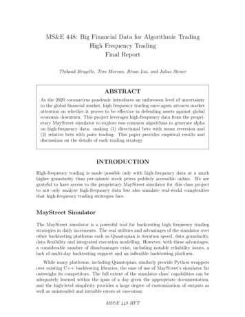
7Short-term window size 0607080Window size of long-term mean9010Short-term window size 5010.03040506070809085.062.5PNLPNL20Window size of long-term meanShort-term window size 907.50.02.5425.07.510.0Short-term window size 300.001020304050607080Window size of long-term mean901020304050607080Window size of long-term mean90Figure 4: Hyper-parameter tuning of two hyperparameters - short-term and long-termwindow sizes - to maximize the end-of-day PnL (USD). Notice that the mean-versionperformance varies largely as the window sizes change slightly, to the extent that thePnL may even be higher when the short-term window size surpasses the long-termone.By tuning the two hyper-parameters, short-term and long-term window sizes, asin Figure 4, we see the PnL of our mean-reversion algorithm largely depends on thewindow sizes, and can flip its sign just by a slight change in the window sizes.Portfolio ConstructionOur mean-reversion algorithm, compared to pairs trading, has the advantage of trading every single ticker in a self-contained fashion, making directional bets on eachticker over time instead of relative bets among tickers. This makes trading a portfoliousing mean reversion as easy as trading each ticker individually and combining theirPnLs.Within each ticker, since we have to clear our position at the end of each pair ofconsecutive, opposite cross-overs, in our mean-reversion strategy, the order size wespecify whenever we buy or sell the ticker at a cross-over determines our inventorydynamics of the ticker. We set the maximum allowable nominal amount for eachorder, and cap the order size according to this product amount as if the order wereexecuted at the mid-price.MS&E 448 HFT

8PNL (USD) over timePNL (USD) over 012:30:0040PNL (USD) over time001020304050607011:06:4020PNLPNL0Figure 5: When trading on a portfolio consisting of {AAPL, CSCO, MSFT, SPY,TSLA, LMT, BA, MRCY, AAN, AAOI, AAON, AAT, AAWW, ABG, ABCB, ABM},ourmean-reversion strategy improves its end-of-day PnL performance as the short-termand long-term window sizes change from (30, 10) (- 51.23, with - 0.213 per trade),to (90, 30) (- 45.30, with - 0.768 per trade), and to (90, 10) (- 16.59, with- 0.180 per trade).We are also aware of another formulation of mean reversion which offers a portfoliowide strategy. In this alternative strategy, the algorithm buys the lower 20% performing stocks in the portfolio and sells the upper 20% performing stocks, anticipatingthe under-performing assets will do better in the future while the over-performingones will ultimately lose their edge over time. This idea leverages the hypotheticalexistence of a portfolio-wide mean each asset should revert to in case they deviatefrom the market, and features a more interesting variety of portfolio weights we canassign to each asset.We present our end-of-day PnL performance of our mean-reversion strategy on acustom portfolio contained inside the Russell 2000 universe in Figure 5.Risk Management PhilosophyTo measure the risk of our algorithm, we track the maximum drawdown and samplevariance of the PnL across time. However, these measures of risk are dwarfed insignificance by the huge dependence of the end-of-day PnL on the short-term andlong-term window sizes, as presented in Figure 4.This phenomenon can be interpreted in the following way. As we decrease thewindow size of any moving average, the resultant moving average becomes less smoothand has more fluctuations, which increases the chance of crossings between the currentand other moving averages. New crossings may emerge and existing crossings maydisappear in a discontinuous manner as we increase the window size of either movingaverage bit by bit. Since we make a new trade and hence a partial contribution to thegrand PnL for every pair of consecutive, opposite cross-overs, the discrete emergenceand disappearance of cross-overs also cause sudden jumps in the PnL. There is noguarantee that these jumps are always positive or negative. This explains the hugereliance of our algorithm’s performance on the window sizes, as predicted above.MS&E 448 HFT

9To solve this issue, one may smoothen out the sudden emergence and disappearance of cross-overs by setting a new, non-negative hyperparameter called themargin. When the margin is zero, this new algorithm reduces back to our originalmean-reversion paradigm. Suppose the margin is positive. Then, we buy the tickeronly when the short-term moving average is at least such a margin below the longterm moving average, and sell the ticker only when the short-term moving averageis at least such a margin above the long-term moving average. Since we are alteringthe trading criteria from discrete time instants at the cross-over points to a range oftime instants, this change will allow for softer entry and exit points throughout theentire trading day, and enables more variety over the order sizes and net positionswe take in each ticker. In this way, we may be able to shift part of the PnL’s heavydependence on the window sizes to a new hyperparameter, the non-negative margin,which is a single scalar easier to optimize over, even for each fixed sub-optimal pairof short-term and long-term window sizes.Execution DiscussionAs mentioned in our MayStreet simulator section, the simulator was unfortunatelybroken for the penultimate week of the quarter. While we had implemented andbacktested crude, signal-less strategies prior to this date, the lack of data or accessto our strategies provided our team with a chance to reflect on the best ways tooptimize our portfolio as well as find consistent sources of alpha. For mean reversion,we developed an interest in utilizing two strategies: grid search and discrete-actionspace reinforcement learning.A grid search involved exploring the low-dimensionality set of high-dimensionalhyperparameters and was relatively simple to implement. However, grid search lacksthe ability to train to an optimum and is inherently slower than other methods oftuning hyperparameters. A typical execution of the simulation can take anywherefrom 30-60 seconds per day of backtesting depending on the parameters given theevent space tracked. Couple the time to execute and the large dimensionality of thehyperparameters themselves (theoretically infinite), the time to execute across all1420 tickers with 3 random trials of length 2 days across 19 different short/long meanlengths and 10 time intervals is conservatively 560 days. Therefore, we ran a subsetof 14 tickers (representing just 1%) which took a little under 6 days. At the end of6 days and within those 14 tickers, there were no consistently profitable assets formean reversion across all 3 random trials. Furthermore, while we recorded the 5 mostprofitable hyperparameter values, they did not appear to be convex or approachinga global optimum.A second potential solution is to use discrete-action-space reinforcement learningas a hyperparameter tuning technique. In theory, a reinforcement learning implementation such as DQN or DDQN could find the optimum hyperparameters due tothe innate ability of RL implementations to perform in high-dimensionality actionspaces. In this case, the state would be the underlying 1st-level metrics of the asset,MS&E 448 HFT

10for example previous day sharpe ratio, volume, etc., and the action would be the setof hyperparameters. However, the involved assumption is that the underlying data isconvex and can be reduced to an optimum. Under this assumption, our grid searchshould have turned out a relatively convex set of optimums, but, as discussed above,this was not the case. Therefore, this cannot be taken as a valid means of tuninghyperparameters for mean reversion on this investment universe.Retrospective DiscussionAll in all, the aim of our implementation of a mean reversal strategy was to determinethe viability of mean reversal in an intra-day/ high frequency trading application.Throughout the roughly 6 weeks we had working access to the simulator, we developed a clear understanding of the inherent difficulties of high frequency trading, andthe extreme variability in returns based on many hyperparameter settings (discussedabove). Within that context and while more study is needed, we believe that consistent profitability using mean reversion in high frequency trading is attempting tosolve for an optimum within a non-convex function. In other words, finding a set ofhyperparameters in a specific investment universe which are consistently profitableis more likely to be the result of careful choices for these hyperparameters than ofstatistics-driven optimizations.2. PAIRS TRADINGThe goal of this strategy is to identify pairs of stocks that show similar price patternsand to benefit from small divergences from this pattern. The strategy itself canbe divided in two separate parts: pair selection and pairs trading. In the pairselection phase, we regress a basket of stocks on the S&P 500 returns and derive theintrinsic stock returns (uncorrelated from the market). We then perform a PCA onthe residuals to identify similar stocks. During the trading phase, we track the spreadof selected pairs and compute running statistics to identify positive trading signals.We typically expect to hold little inventory of stocks, and to have the strategy runningevery day during market hours.Investment Universe SelectionOne of the most important parts of the pairs trading strategy is to find a pair of assetsthat will be relevant. We spent a lot of time picking the right pairs and used severalmethods for this purpose. Among the strategies that we use for the pairs selection, wewill discuss a statistical-based methodology and more experimental machine-learningbased approach. The latter is only to confirm or disprove the conclusions from thestatistical-based methods that were used to select consistent pairs of stocks.MayStreet provided us high-frequency data so we used these data to select the pairs.MS&E 448 HFT

11It is primordial to look at stocks that have similar properties and features on a dailybasis. However, in order to make consistent choices, it is also very important toaggregate the results obtained on a daily basis to a larger scale.Pairs Selection MethodologyThe technical details and results of the selection are described in the Modelingsection.1. Choose a broad portfolio of stocks from different industries.2. Pick a random trading day and retrieve the data from this day.3. Statistical Analysis to get an idea of potential pairs.4. For each potential pairs, we compute relevant metrics and perform several statistical tests with given thresholds. To illustrate, we compute the correlation orthe Hurst exponent, and then we perform an Engle– Granger two-step methodfor testing the correlation.5. Get rid of the pairs that fail the tests or that are above our thresholds.6. Restart step 2 with the remaining pairs.After applying this methodology to our portfolio, we applied unsupervised learningmethods to confirm or disprove our results. Precisely, we used clustering methods suchas K-means and Affinity Propagation. The advantage of using these two methodsis the ability to use two different distance matrices. K-Means model is built uponEuclidean distance but it makes more sense to use the correlation matrix as a distancesince we work with time series: this is why we also used the Affinity Propagationalgorithm.Finally, we included in our strategy some pairs from the same industry such as Visaand MasterCard or JPMorgan and Morgan Stanley but we also made less intuitiveassociations such as Apple with Mastercard or Apple with Goldman Sachs. The waya pair was traded is described in the Portfolio Construction section.ModelingFirst, let us illustrate what statistical analysis methods were performed in orderto understand the data we had. Principal Component Analysis (PCA) is a goodstatistical model to observe correlation patterns within a portfolio. In order to makean analysis of the returns series Rt , we used SPDR S&P 500 returns Mt to computethe linear regression :Rt βMt α tMS&E 448 HFT

12Figure 6: AAPL returns against MarketThe idea is to get the intrinsic properties of the stocks returns without the marketinfluence. This is why we applied the PCA framework to the residuals returns in ourportfolio ( t )t .Figure 8Figure 7From the results above, we can notice that there exists several correlation patternswithin our portfolio. These patterns are mostly clustered by industry. It gives us anidea of potential pairs that are close enough to build an efficient strategy. Furthermore, the Affinity Propagation algorithm can provide information from a differentperspective depending on the distance matrix used.MS&E 448 HFT

13Figure 9: Affinity Propagation clustering with PCA dimensionality reductionIn this case, we see that AAPL and MA are clustered together but the clustersare not based on the correlation relationships between the stocks. By considering thefact that Apple introduced its Apple Card recently, by working with Goldman Sachsand Mastercard, we could take advantage of this collaborative association to createa less intuitive pair.Second, let us describe some of the metrics and tests used to make a precise pairsselection. In order to know if a stock has mean reversal properties, we used the Hurstexponent as described in the Mean Reversion sections. Furthermore, once two stocksare pre-selected as a potential pair, we compute the Pearson correlation coefficientwhich measures how the securities move together. For two stocks A and B, this metricis given by:cov(XA , XB )ρA,B σXA σXBThen the second step is to test for co-integration between the stocks. For this purpose,we used the Granger – Engel test to check if two series xt , yt are cointegrated, ie, whenthe distance between them does not change drastically over time. The test assumesthat xt , yt I(1) so we used a ADF test to show that the first difference of xt andyt are stationary. Then it tests for ut I(0) in the model : yt α βxt ut . Twoco-integrated stocks were a very good candidate to bulild a pair and usually it wasour last criteria to do the pair selection.Portfolio ConstructionOnce a pair is identified (e.g. Visa vs. Mastercard), we create a synthetic asset S onwhich we will trade for the day:S n1 S1 n2 S2MS&E 448 HFT

14With (S1 , S2 ) the pair of stocks selected, and (n1 , n2 ) N 2 such that Trade nominal ni roundOpen mid price of SiTrade nominal is a model parameter that will be discussed in the next sections.Through this definition, S becomes a vehicle of all the relevant information to monitorby our strategy. By defining (n1 , n2 ) in this manner, we ensure that: P rice(S) 0. Cash balance 0, e.g. we have little to no cash flow when we enter a trade. S is uncorrelated to market movements. Cash borrow costs become negligible compared to equity borrow costs.Alpha ModelingOur first approach was to model our asset S by a N (µS , σS2 ) law, and to derive ourtrading signals on the position of S with regards to (µS , σS2 ). Our first challengewas to have an accurate measure of these two statistics throughout the trading day.We opted for window based statistics, and computed the running sample mean andvariance based on two parameters: Time-interval: Time interval at which we request market data, compute statistics and send trade orders.Typical Value: 1 second Window-size: Number of time intervals on which define the sample for statistics computation.Typical Value: 300We then define:S µSσSand look at the position of the time-series based on a third parameter:Z Threshold: Multiple of σS serving as trigger for trading signals.Typical Value: 2The alpha signals were then directly derived from this threshold value: If S threshold Sell S If S threshold Buy SMS&E 448 HFT

15Figure 10Figure 11Risk Management PhilosophyWe identified multiple sources of risk in out strategy:Execution RiskAs MayStreet provides a realistic HFT order management system, we were confrontedby the execution risks of automated strategies. To prevent the realization of spurioustrades, we limited ourselves to market limit orders hitting the first level of the orderbook. When our trades were not fully executed by the next time interval due toslippage or partial fill, we would cancel all outgoing orders and send new trades if thesignal was still present.Regulatory RiskTo ensure that our activity was compliant with market regulations, we monitored ourfill ratio :number of orders filledfill ratio number of orders sentwhich widely passed exchanges requirements. As we were only removing liquidityfrom the order book, we were safeguarded from spoofing and blinking behav

MS&E 448: Big Financial Data for Algorithmic Trading High Frequency Trading Final Report Thibaud Bruyelle, Tom Morvan, Brian Lui, and Julius Stener . The plot highlights just the rst level of the order book, but the simula-tor a orded us access to every existing level