Transcription
An Introduction to Computer Programming(with MATLAB) for Scientific ComputingWeizhang Huang1January 15, 20201Department of Mathematics, The University of Kansas, Lawrence, KS 66045 USA.
ii
PrefaceThese notes are prepared for students with basic knowledge on calculus and matrix theory.Students are not required to have prior knowledge on the numerical methods discussed inthese notes. Students who are interested in numerical analysis and scientific computingare encouraged to take courses and/or read textbooks in the area. An example is Burden,Faires, and Burden [1].iii
iv
ContentsPrefaceiii1 Programming Basics1.1 Decimal and binary number systems and conversion1.2 Common components among computer languages . .1.2.1 Data types . . . . . . . . . . . . . . . . . . .1.2.2 Basic operators . . . . . . . . . . . . . . . . .1.2.3 Selection and loop statements . . . . . . . . .1.2.4 Functions . . . . . . . . . . . . . . . . . . . .1.3 Flowchart . . . . . . . . . . . . . . . . . . . . . . . 352 An2.12.22.32.42.52.62.7Introduction to MATLABData representations and typesArithmetic operations . . . . .Relational and logical operatorsSelection and loop statements .Functions . . . . . . . . . . . .How to plot data in MATLABA few functions useful to know.3 Lab3.13.23.33.43.51: Convert DecimalProblem description .Planning . . . . . . . .Coding . . . . . . . . .Testing . . . . . . . .Reporting . . . . . . .4 Lab4.14.24.34.42: Piecewise Linear Interpolation forProblem description . . . . . . . . . . . .Planning . . . . . . . . . . . . . . . . . . .Coding . . . . . . . . . . . . . . . . . . . .Testing . . . . . . . . . . . . . . . . . . .Numbers into Binary. . . . . . . . . . . . . . . . . . . . . . . . . . . . . . . . . . . . . . . . . . . . . . . . . . . . . . . . . . . . . . . . . .va.Form. . . . . . . . . . . . . . . .Given Data. . . . . . . . . . . . . . . . . . . . . . . . . . . . .Set. . . . . . . . .
CONTENTS15 Lab5.15.25.35.43: The Method of Least SquaresProblem description . . . . . . . . .Planning . . . . . . . . . . . . . . . .Coding . . . . . . . . . . . . . . . . .Testing . . . . . . . . . . . . . . . .37373939406 Lab6.16.26.36.46.54: The Composite Gauss-Legendre QuadratureProblem description . . . . . . . . . . . . . . . . . . .Planning . . . . . . . . . . . . . . . . . . . . . . . . . .Coding . . . . . . . . . . . . . . . . . . . . . . . . . . .Testing . . . . . . . . . . . . . . . . . . . . . . . . . .The composite Simpson’s rule . . . . . . . . . . . . . .4141444445467 Lab7.17.27.37.47.55: Euler’s Scheme for Solving Ordinary Differential EquationsProblem description . . . . . . . . . . . . . . . . . . . . . . . . . . . . .Planning . . . . . . . . . . . . . . . . . . . . . . . . . . . . . . . . . . . .Coding . . . . . . . . . . . . . . . . . . . . . . . . . . . . . . . . . . . . .Testing . . . . . . . . . . . . . . . . . . . . . . . . . . . . . . . . . . . .Heun’s and RK4 schemes . . . . . . . . . . . . . . . . . . . . . . . . . .494950515151Bibliography.52
2CONTENTS
Chapter 1Programming BasicsIn this chapter we study programming basics, including decimal and binary number systemsand their conversion, floating-point number representations in a computer, and commoncomponents among computer languages.1.1Decimal and binary number systems and conversionNumbers we use in daily life are called decimal numbers. Examples include 0, 12, 3.1415926and 1234.56. Take 1234.56 as an example. We know that 1 is the digit for thousands,2 for hundreds, 3 for tens, 4 for ones, 5 for tenths, and 6 for hundredths. Indeed, thenumber is read as one thousand two hundred thirty four point five six. Translating this intomathematics, we can express the number into a series of powers of 10, i.e.,1234.56 1 103 2 102 3 101 4 100 5 11 6 2.11010For this reason, decimal numbers are also called base-10 numbers. The digits we use are 0,1, ., and 9.On the other hand, most modern computers use the so-called binary number system,which uses base 2 and the digits 0 and 1. An example is 11011.01. To distinguish numbers in binary and decimal systems, we denote 11011.01 in the binary number system by(11011.01)2 . It can be expressed into a series of powers of 2 as(11011.01)2 1 24 1 23 0 22 1 21 1 20 0 11 1 2.212This explains the meanings of the digits. Moreover, it can be used to convert a binarynumber into a decimal number. Indeed, carrying out the calculations of the right-hand sideterms, we have(11011.01)2 16 8 0 2 1 0 0.25 27.25Exercise 1.1.1. Convert the following binary numbers into decimal numbers: (1010101)2 ,(111)2 , and (0)2 .3
4CHAPTER 1. PROGRAMMING BASICSIn the following example we explain how to convert decimal numbers into binary form.Example 1.1.1. Convert x 11 into binary form.Since 23 x 24 , we know that x can be expressed asx a 23 b 22 c 21 d 20 ,where a 1 and b, c, and d are to be determined. From the above expression, we havex 1 23 b 22 c 21 d 20 .On the other hand, x 1 23 11 1 23 3. Recall that b can take 0 or 1. If b 1, thenthe right-hand side of the above equation is at least 4, which is greater than the left-handside whose value is 3. Thus, b must be zero. With this, we havex 1 23 0 22 c 21 d 20andx 1 23 0 22 11 1 23 0 22 3.Comparing these equations, we get c 1. Inserting this into the above two equations yieldsx 1 23 0 22 1 21 d 20 ,x 1 23 0 22 1 21 11 1 23 0 22 1 21 1,which lead to d 1. Thus, we obtain11 (1011)2 .Now we use a slightly different procedure. First, we find the integer m such that2m 1 x 11 2m .It is not difficult to see m 4. Then, x can be expressed as 1111x a 1 b 2 c 3 d 4 24 (0.abcd)2 24 .2222The values of a, b, c, and d are to be determined.Define x0 x 2 4 . Then, x0 11 2 4 11/16 and 2x0 22/16 11/8. Moreover,2x0 has the expression1112x0 a b 1 c 2 d 3 .222Since 2x0 1, we know that a 1.Next, we define x1 2x0 1. We can find that x1 11/8 1 3/8 and the expressionof 2x1 is112x1 b c 1 d 2 .22
1.1. DECIMAL AND BINARY NUMBER SYSTEMS AND CONVERSION5Since 2x1 6/8 1, we have b 0.Repeating this process, we can find c 1 and d 1. Thus, we obtain the binary formof 11 is11 (0.1011)2 24 ,which is the same as what we obtained before.The second procedure is summarized in Table 1.1.Table 1.1: The summary of the second procedure to convert x 11 into binary form.xnx0x1x2x3x4test2 4 x 11/16 2x0 a 3/8 2x1 b 3/4 2x2 c 1/2 2x3 d 02x02x12x22x32x4binary digits 22/16 1 6/8 1 6/4 1 1 1 0a 1b 0c 1d 1computation stopsExercise 1.1.2. Convert the following decimal numbers into binary form using the procedure shown in Table 1.1: 15, 3.25, 8 and 4.When x is nonzero, there exists an integer m such that 2m 1 x 2m . Then, x canbe expressed as 111x a1 1 a2 2 · · · an n · · · 2m(1.1)222 (0.a1 a2 · · · an · · · )2 2m ,(1.2)where a1 1 and an 0 or 1 for n 2, 3, . Moreover, the procedure in Table 1.1 can betranslated into Algorithm 1.1.1 to convert any nonzero decimal number into binary form(1.2).Exercise 1.1.3. Explain why the zero cannot be expressed into the form (1.2).Exercise 1.1.4. Explain why a1 1 in the binary form (1.2) for any nonzero decimalnumber.Exercise 1.1.5. Show that Step 2(a) of Algorithm 1.1.1 is correct for n 1.Interestingly, (1.2) can be used to show how (real) numbers are represented in a computer. We first notice that a computer has a finite amount of storage units so a (real)number on a computer can only have a finite number of fractional digits (called the mantissa) and its exponent m is in a bounded range. Thus, a number in a computer lookslikex (0.a1 a2 · · · an )2 2m ,(1.3)
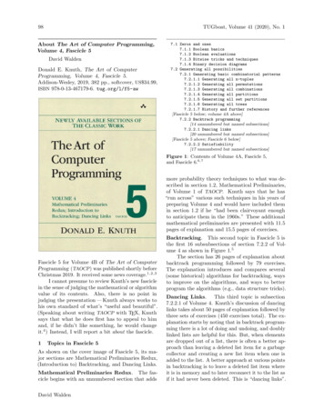
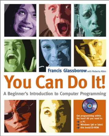
6CHAPTER 1. PROGRAMMING BASICSAlgorithm 1.1.1 Convert nonzero decimal numbers into the binary form (1.2).1. Initialization: Determine the sign of x and the integer m such that 2m 1 x 2m .Set x0 x 2 m .2. For n 1, 2, · · · do(a). If 2xn 1 1, set an 1; otherwise, an 0.(b). Compute xn 2xn 1 an .(c). If xn 0, stop the computation.where n is a positive integer, a1 1, and m (which is also saved in binary form) is aninteger in a bounded range. Each of the digits is stored in a bit, with 8 bits being groupedinto a byte. As an example, we now consider two most common number representations in acomputer. According to the 754-2008 standard of the Institute of Electrical and ElectronicsEngineers (IEEE), the 32-bit floating-point format (single precision) uses 1 bit for sign, 23 bits for the mantissa (and n 24), 8 bits for the exponent.This is shown in Fig. 1.1. One may notice that a1 is not saved since it is known to be 1for any nonzero number. Moreover, the largest integer that can be stored for the exponentis (11111111)2 255. In order to represent negative exponents, the actual exponent isobtained by subtracting 127 from what is stored in the exponent part. Thus, the bits areconverted into a numeric value as sign (0.1 mantissa )2 2 exponent 127 .Note that zero cannot be expressed in the above form. Special specifications are defined forzero and several other special values including NaN (Not a Number). 8 bitsfor exponent123 bitsfor mantissaFigure 1.1: IEEE 754-2008 format for 32-bit floating-point numbers.The IEEE 754-2008 specification of 64-bit floating-point (double precision) numbers isshown in Fig. 1.2. The bits are converted into a numeric value as sign (0.1 mantissa )2 2 exponent 1023 .
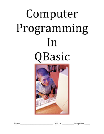
1.2. COMMON COMPONENTS AMONG COMPUTER LANGUAGES 11 bitsfor exponent752 bitsfor mantissa1Figure 1.2: IEEE 754-2008 format for 64-bit floating-point numbers.To conclude this section, we take a look at basic hardware of a computer; see Fig. 1.3.The central processing unit (CPU) is the brain of a computer, which carries out all of basicoperations on data. Data are transferred between CPU and the main memory and betweenthe main memory and the hard disk. It is pointed out that numbers are stored and operatedin CPU using more bits than they are stored in the main memory or the hard disk. Roundofferror can occur when they are transferred between CPU and the main memory. Roundofferror can also occur when numbers have longer fractional digits than those in the mantissa.Although it is very small ( 10 16 for double precision), roundoff error can accumulate andbe amplified greatly when algorithms are not carefully designed (in this case the algorithmsare unstable) or the problem at hand is ill-conditioned. While stability of algorithms andconditioning of problems are two important topics considered in scientific computing, wewill not go into detail due to the scope of this course.CPUInputMain MemoryDevicesOutputDevicesHard DiskFigure 1.3: Basic hardware for a computer.1.2Common components among computer languagesComputer CPUs only understand instructions written in binary (machine code). It is extremely difficult for humans to write programs in machine code. Computer languages havebeen developed over the years so people can write programs more easily. Those languagesserve more or less as translators that translate what people write into something computers
8CHAPTER 1. PROGRAMMING BASICSunderstand. Commonly used computer languages include C, C , Fortran, Visual Basic,Python, and JavaScript. In this course, we will focus on MATLAB1 , which “combines adesktop environment tuned for iterative analysis and design processes with a programminglanguage that expresses matrix and array mathematics directly” (as quoted from the MATLAB website). Another very useful language is R, which is also a combined language andenvironment but is used more for statistical computing and graphics.High-level computer languages share many common features. In this section we overviewsome of those features, including data types, basic operators, selection and loop statements,and functions. These features will be discussed in detail in the next chapter for MATLAB.1.2.1Data typesData types are classifications that specify what variables or objects can hold in programming, and must be referenced and used correctly. Common examples of data types are Float (for single precision real numbers; recall from the previous section that singleprecision numbers usually occupy 32 bits in computer memory) Double (for double precision real numbers; recall from the previous section that singleprecision numbers usually occupy 64 bits in computer memory) Integer (for integer numbers) Character (for single characters such as a, 4) String (for groups of characters such as abcd, a3c4#) Boolean (true or false)1.2.2Basic operatorsEach computer language provides a number of operators. Common examples of basic operators are Assignment Operators are used to assign the result of an expression to a variable.For example,variable expressionmeans that the computer evaluates the expression on the right-hand side and thenstores the result in the memory unit assigned to the left-hand side variable. Languagesmay provide various shorthand assignment operators. Arithmetic Operators: (addition), - (subtraction), * (multiplication), and /(division). Many languages also provide modulo division.1MATLAB R is a trademark of The MathWorks, Inc., Natick, MA 01760.
1.2. COMMON COMPONENTS AMONG COMPUTER LANGUAGES9 Relational Operators are used to make comparison: (less than), (less than orequal to), (greater than), (greater than or equal to), (equal to), and ! or (not equal to). Logical Operators are used when more than one conditions are to be tested: &&(logical AND), (logical OR), ! or (logical NOT). The result of any logicalexpression is either TRUE or FALSE.1.2.3Selection and loop statementsIn addition to assignment statements, most commonly used statements include selection andloop statements. Brief information and basic formats of these statements are given here.Detailed explanation and examples for the selection and loop statements in MATLAB willbe given in §2.4.A selection statement selects among a set of statements depending on the value of acontrolling expression. Selection statements typically include if and switch statements.Their syntaxes look likeif (conditional-expression){statements}elseif (conditional-expression) (optional){statements}else (optional){statements}switch (expression)case (constant-expression){statements}.default: (optional){statements}
10CHAPTER 1. PROGRAMMING BASICSCommon examples of loops include for and while loops. Their syntaxes looks likefor (initialization Statement; test Expression; increment Statement){statements}initialization statementwhile (condition){statementsincrement/decrement statement}The break statement is often used with loop statements to break the loop.1.2.4FunctionsEach computer language provides a large set of functions including elementary functions inmathematics. At the same time, it also allows us to define our own functions. Generallyspeaking, this can be done inline (embedded in the code) or in file (programs in file). Inaddition to the rules for defining these functions, we need to pay special attention to thescope of the functions in file, for instance, where functions are visible, in the same file orin the same folder, public or private. See §2.5 for MATLAB functions.1.3FlowchartFlowchart is a graphical representation of an algorithm. It is a very useful tool to plan aprogram because it indicates the flow and steps of information and processing. Flowchartsare used in analyzing, designing, documenting or managing a process or program in variousfields.Here we do not attempt to learn how to draw flowcharts using common symbols. Instead,we want to emphasize the importance of planning (steps and flow) for an algorithmbefore we begin to write the code. We will address this issue in every lab.
Chapter 2An Introduction to MATLABMATLAB, standing for MATrix LABoratory, combines an interactive desktop environmentwith a matrix-based computer language and provides an abundance of built-in commands,math functions, and tool boxes for numerical computation, visualization, and programming.This chapter presents an introduction to MATLAB. We study its basics such as data types,arithmetic operations, relational operations, selection and loop statements, functions, andgraphics. Our goal is to get ourself ready in a reasonably short time for further studiesof programming principles for scientific computing in later chapters. It is worth remindingthat the best way to learn a computer language is with our hands. So try as many examplesas possible on the computer.2.1Data representations and typesMATLAB needs to be installed on the computer you will be using. After it is installed, youcan start MATLAB by double clicking its icon.Once MATLAB is started, you can find the command window with the prompt sign .Then try commands pwd and help. (In the following block, the left column are MATLABcommands while the right columns are explanations.) pwd help help help plotThis shows the path of the current directory/folderThis gets help for helpThis gets help for plotNote that MATLAB is case-sensitive. For example, plot is different from Plot.A distinct feature of MATLAB (from many other languages such as C or C ) is thatthere is no need to declare data types for variables before their use. A variable’s data typeis determined from its first assignment. Nevertheless, it is often more efficient (in termsof memory use and CPU time) to preallocate arrays (including vectors and matrices) before their first use. This can be done by assignment statements. For example, the command11
12CHAPTER 2. AN INTRODUCTION TO MATLAB A zeros(100, 200);preallocates a 100-by-200 block of memory for variable A and initializes it to be zero.MATLAB’s data representations are all interpretations of one basic structure, the matrix. This is a rectangular array of numbers, stored and manipulated internally using thecomputer’s floating point format and operations. The basic matrix data structure can havespecial interpretations in a number of situations. x 3.14; x 3.14 v [1, 2, 3, 4]; v [1 2 3 4]; u [1; 2; 3; 4]; A [1, 2; 3, 4];b 0.3 0.4*i;C [0.1 0.2; 0.3 0.4] . [0.5 0.6; 0.7 0.8]*i;ch ’a’; st ’Hello World’; sm [’Hello’; ’World’]; aa {’a’, 2; ’b’, 3};x is a real number (a 1-by-1 matrix)(double precision by default)what is the difference?v is a row vector(or a 1-by-4 matrix)what is the difference?u is a column vector(or a 4-by-1 matrix)A is a 2-by-2 matrixb is a complex numberwhat . is used for?C is a complex matrixThis creates a character ’a’ andassigns it to variable chst is a string or a character arraysm is a string matrixaa is a cell that uses { }It is important to point out that while being displayed according to their defined sizesand shapes, arrays are actually stored in memory as a single column of elements. Considerthe matrix 1 2 3 A 4 5 6 .7 8 9Matrix A can be accessed via matrix indexing as A(3, 2) 8. On the other hand, matricesare actually stored column by column; in other words, A is stored in memory as a vectorcontaining the sequence of elements 1, 4, 7, 2, 5, 8, 3, 6, 9. As a result, A can also be accessedvia the so-called linear indexing (denoted as A(:)); for example, we have A(2) 4 andA(6) 8. Understanding how matrices are stored in memory is often useful in making thecode more efficient in implementation.The MATLAB data types commonly used in scientific computing are listed as follows. Numeric Types include integers, floating-point data (single precision, double preci-
2.2. ARITHMETIC OPERATIONS13sion (default), and complex). Logical Data Type represents true or false states using the numbers 1 and 0,respectively. Characters and Strings include character arrays such as c ’Hello World’ andstring arrays, such as str "Greetings friend". Cell Arrays are arrays that can contain data of varying types and sizes, such asmyCell {1, 2, 3; ’text’, rand(5,10,2), {11; 22; 33}}. Structures are arrays with named fields that can contain data of varying types andsizes, such as s.a 1; s.b {’A’,’B’,’C’}; Function Handles: A function handle is a data type that stores an association toa function. To create a handle for a function, precede the function name with an @sign. For example, if we have a function called myfunction, we can create a handlenamed f as: f @myfunction;Exercise 2.1.1. Give two examples of variables in each of numeric, logical, character,and cell types.2.2Arithmetic operationsMATLAB has two different types of arithmetic operations: matrix operations and arrayoperations. They are used to perform numeric computations, for example, adding twonumbers, raising the elements of an array to a given power, or multiplying two matrices.Matrix operations follow the rules of linear algebra. (matrix addition) and - (matrix subtraction). Although they are named matrixaddition and subtraction, they should be more precisely called array addition andsubtraction (see discussion on array operations below). On the one hand, they actlike ordinary matrix addition and subtraction when the operands have the same size.For example,2 3 5[1, 2; 3, 4] - [5, 6; 7, 8] [-4, -4; -4, -4]On the other hand, when operands have compatible sizes but not necessarily thesame size each input is implicitly expanded as needed to match the size of the otherduring execution of the computation. We give several examples in the following. Thereader can find more information on compatible sizes by searching Compatible ArraySizes for Basic Operations.
14CHAPTER 2. AN INTRODUCTION TO MATLAB(1) 10 [1, 2; 3, 4] In this example, the first operand is expanded into [10,10; 10, 10] to match the size of the second operand during execution of thecalculation. Thus, we have"#"# "# "#1 210 101 211 1210 3 410 103 413 14(2) [1, 2; 3, 4] 10 The second operand is expanded into [10, 10; 10, 10]to match the size of the first operand during execution of the calculation, i.e.,"#"# "# "#1 210 1011 121 2 10 3 43 410 1013 14(3) [1, 2; 3, 4] [5, 6] The second operand is expanded into [5, 6; 5, 6]to match the size of the first operand during execution of the calculation. Thisgives"#"# "# "#hi1 21 25 66 8 5 6 3 43 45 68 10(4) [1, 2; 3, 4] [5; 7] The second operand is expanded into [5, 5; 7, 7]to match the size of the first operand during execution of the calculation, whichyields"# " #"# "# "#1 251 25 56 7 3 473 47 710 11(5) [1;2;3] [1, 2; 3, 4] The operands do not have compatible sizes. *: multiplication. It works for matrices under the rules of linear algebra, with scalarsand vectors being considered as special forms of matrices. For example, A*B makessense when the number of columns of A is equal to the number of rows of B. Forany scalar alpha, alpha*A or A*alpha is a standard multiplication of matrices andscalars. For examples,[1, 2; 3, 4]*5 [5, 10; 15, 20][1, 2; 3, 4]*[5, 6] (error using *)[1, 2; 3, 4]*[5; 6] [17; 39][1, 2; 3, 4]*[5, 6; 7, 8] [19, 22; 43, 50] /: right division. This is used mostly for scalars, i.e., a scalar divided by anotherscalar, for example,3/4 0.75(2*10)/5 4It can also be used for matrices (although rare), for example, A/B is calculated via(A’\B’)’, where ’ is the matrix transpose and \ is the left division that is to beexplained below.
2.2. ARITHMETIC OPERATIONS15 : power. For example, 3.1 2.5 represents the 2.5th power of 3.1. Note that the3rd power of -2 should be expressed as (-2) 3. Moreover, A 2.1 stands for the 2.1thpower of matrix A. For example,[1, 3; 2, 1] 2 [7, 6; 4, 7] \: Backslash or left matrix divide. A\B is the matrix division of A into B, which isroughly the same as INV(A)*B, except it is computed in a different way. If A is anm-by-n matrix with m n or m n and B is a column vector with m components,or a matrix with several such columns, then A\B is the solution in the least squaressense to the under- or overdetermined system of linear system Ax B. For example,"#" # " #1 2x13 .1 1 x20The solution for this system is given byx [1, 2; 1, -1]\[3; 0] [1; 1]On the other hand, array operations execute element by element operations oncorresponding elements of vectors, matrices, and multidimensional arrays. More specifically,if the operands have the same size, then each element in the first operand gets matchedup with the element in the same location in the second operand. If the operands havecompatible sizes, then each input is implicitly expanded as needed to match the size of theother. The period character “.” distinguishes array operations from matrix operations.Moreover, MATLAB does not provide . and .- because, as mentioned above, and already serve as array addition and subtraction. .*: array multiplication.[1, 2; 3, 4].*[5, 6; 7, 8] [5, 12; 21, 32][1, 2; 3, 4].*[5, 6] [5, 12; 15, 24]In this example, the second operand is expanded into [5, 6; 5, 6] to match the sizeof the first operand during execution of multiplication.[1, 2; 3, 4].*[5; 7] [5, 10; 21, 28]In this example, the second operand is expanded into [5, 5; 7, 7] to match the sizeof the first operand during execution of the calculation. ./: right-array division. This operation is similar to the array multiplication. Forexample,[1, 2; 3, 4]./[5; 7] [1/5, 2/5; 3/7, 4/7]where the second operand is expanded into [5, 5; 7, 7] to match the size of thefirst operand. . : array power. This operation is similar to the array multiplication. For example,[1, 2; 3, 4]. [5; 7] [1 5, 2 5; 3 7, 4 7]where the second operand is expanded into [5, 5; 7, 7] to match the size of the first
16CHAPTER 2. AN INTRODUCTION TO MATLABoperand. [1, 2; 3, 4]. 3 [1 3, 2 3; 3 3, 4 3] where the second operand isexpanded into [3, 3; 3, 3] to match the size of the first operand.Exercise 2.2.1. Do the calculations by hand and check your answers with MATLAB.(1) [1, 2; 3, 4] - 20 and [1, 2; 3, 4] - [1;2](2) [1;2]*[1, 2; 3, 4] and [1;2].*[1, 2; 3, 4](3) [1, 2; 3, 4] 2 and [1, 2; 3, 4]. 2(4) [1;2;3].*[1, 2; 3, 4]Exercise 2.2.2.(1) Solve the following linear system by hand,(x y 15x y 5"orAu b where#1 1,A 1 1"#15b .5(2) Input A and b in MATLAB and then find the solution u using the \ operator. Verifyyour answer with the one obtained by hand.(3) Try inv(A), det(A), [V,D] eig(A), and A’*A. What are they?2.3Relational and logical operatorsThe relational and logical operators perform element-wise comparisons between twoarrays. The arrays must have compatible sizes to facilitate the operation. Arrays with compatible sizes are implicitly expanded to be the same size during execution of the calculation.The entries of the resulting array are either 1 (true) or 0 (false).Relational operators in MATLAB include (less than) (less than or equal to) (greater than) (greater than or equal to) (equal to) (not equal to)For example,
2.3. RELATIONAL AND LOGICAL OPERATORS17 [6, 6; 6, 6] [5, 6; 7, 8] [1, 0; 0, 0] [6, 6; 6, 6] [5, 6] [1, 0; 1, 0] (the second operand is expanded) [6, 6; 6, 6] [5; 6] [1, 1; 0, 0] (the second operand is expanded) [1, 2; 3, 4] 2.5 [0, 0; 1, 1] (the second operand is expanded)The following are commonly used logical operators. & (and): A & B performs a logical AND of arrays A and B and returns an array containingelements set to either logical 1 (true) or logical 0 (false). An element of the outputarray is set to logical 1 if both A and B contain a nonzero element at that same arraylocation. Otherwise, the array element is set to 0. For example,4 & 0 00 & 0 04 & 3 1[1, 2; 1, 0] & [0, -1; 2, 3] [0, 1; 1, 0][1, 2; 1, 0] & [0, -1] [0, 1; 0, 0] (the second operand is expanded)true & false 0 (or): A B performs a logical OR of arrays A and B and returns an array containingelements set to either logical 1 (true) or logical 0 (false). An element of the outputarray is set to logical 1 if either A and B contain a nonzero element at that same arraylocation. Otherwise, the array element is set to 0. For example,4 0 10 0 04 3 1[1, 2; 1, 0] [0, -1; 2, 3] [1, 1; 1, 1][1, 2; 1, 0] [0, -1] [1, 1; 1, 1] (the second operand is expanded)true false 1 (not): A returns a logical array of the same size as A. The array contains logical 1values where A is zero and logical 0 where A is nonzero. For example, [1, 2; 1, 0] [0, 0; 0, 1]Exercise 2.3.1. Compute the following expressions and check your answer with MATLAB.(1) [1, 2; 3, 4] 3(2) [1, 2; 3, 4] [1, 2](3) [1, 2; 3, 4] [1; 3](4) [1, 2; 3, 4] & [0, 5]
18CHAPTER 2. AN INTRODUCTION TO MATLAB(5) [1, 2; 3, 4] [0; 5](6) (3 2) & (1 2)(7) (3 2) (1 2)2.4Selection and loop statementsSelection statements in MATLAB include if and switch statements. The syntax of ifstatement isif conditional-expressionstatementselseif conditional-expression (optional)statementselse (optional)statementsendConsider the step functiony (0,for x 01,for x 0.The if statement for this function isx input(’Enter a number: ’);if x 0y 0;elsey 1;enddisp(y)Here, we have used input and disp. Check out their usage using help.The syntax of switch statement isswitch swi
An Introduction to Computer Programming (with MATLAB) for Scienti c Computing Weizhang Huang1 January 15, 2020 1Department of Mathematics, The University of Kansas, Lawrence, KS 66045 USA. ii. Preface These notes are prepared for stu