Transcription
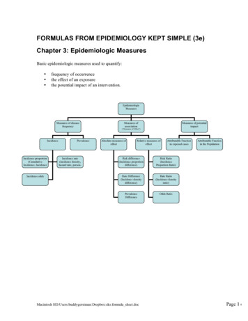
FORMULAS FROM EPIDEMIOLOGY KEPT SIMPLE (3e)Chapter 3: Epidemiologic MeasuresBasic epidemiologic measures used to quantify: frequency of occurrencethe effect of an exposurethe potential impact of an intervention.EpidemiologicMeasuresMeasures of diseasefrequencyIncidenceIncidence proportion(CumulativeIncidence, IncidenceRisk)Incidence oddsPrevalenceIncidence rate(incidence density,hazard rate, persontime rate)Measures ofassociationMeasures of potentialimpact(“Measures of Effect”)Absolute measures ofeffectRelative measures ofeffectAttributable Fractionin exposed casesRisk difference(Incidence proportiondifference)Risk Ratio(IncidenceProportion Ratio)Rate Difference(Incidence densitydifference)Rate Ratio(Incidence densityratio)PrevalenceDifferenceOdds RatioMacintosh HD:Users:buddygerstman:Dropbox:eks:formula sheet.docAttributable Fractionin the PopulationPage 1 of 7
3.1 Measures of Disease FrequencyIncidence Proportion No. of onsetsNo. at risk at beginning of follow-up Also called risk, average risk, and cumulative incidence. Can be measured in cohorts (closed populations) only. Requires follow-up of individuals.Incidence Rate No. of onsets person-time Also called incidence density and average hazard. When disease is rare (incidence proportion 5%), incidence rate incidence proportion. In cohorts (closed populations), it is best to sum individual person-time longitudinally. It can alsobe estimated as Σperson-time (average population size) (duration of follow-up). Actuarialadjustments may be needed when the disease outcome is not rare. In an open populations, Σperson-time (average population size) (duration of follow-up).Examples of incidence rates in open populations include:Crude birth rate (per m) birthsmid-year population sizeCrude mortality rate (per m) Infant mortality rate (per m) Prevalence Proportion mdeathsmid-year population sizedeaths 1 year of agelive births m mNo. of casesNo. of individuals in the study Also called point prevalence or just prevalence. The concept of period prevalence should be avoided when possible because it confuses theconcepts of incidence and prevalence (Elandt-Johnson & Johnson, 1980). Prevalence dependence on the “inflow” and “outflow” of disease according to this formulaPrevalence (incidence rate) (average duration of illness).Additional Notes Terminology: The term “rate” is often used loosely, to refer to any of the above measures ofdisease frequency (even though the only true rate is the incidence density rate Odds: Both prevalence and incidence proportions may be addressed in terms of odds. Let prepresent the incidence proportion or prevalence proportion of disease and o represent the odds ofdisease. Thus, odds o p / (1 – p). Reporting: To report a risk or rate “per m,” simply multiply it by m. For example, an incidenceproportion of 0.0010 0.0010 10,000 10 per 10,000. Uni-cohort: To report a risk or rate as a unicohort, take its reciprocal and report it as 1 in“unicohort.” For example, an incidence proportion of 0.0025 1 inMacintosh HD:Users:buddygerstman:Dropbox:eks:formula sheet.doc10.0025or “1 in 400.”Page 2 of 7
3.2 Measures of Association (Measures of Effect)Notation and terminology: Concepts apply to incidence proportions, incidence rates, and prevalenceproportions, all of which will be loosely called “rates.” Let R1 represent the rate or risk of disease in theexposed group and let R0 represent the rate or risk of disease in the non-exposed group.Absolute Measure of Effect (Rate Difference)RD R1 R0Relative Measure of Effect (Rate Ratio)RR R1R0The relative effect of an exposure can also captured by the SMR (see section on Rate Adjustment)2-by-2 Cross-TabulationE (Group 1)E (Group 0)D A1A0M1D B1B0M0TotalN1N0N For person-time data (incidence rates/densities) ignore cells B1 and B0 and let N1 and N0 representthe person-time in group 1 and group 0, respectively. Rates, Rate Ratio, and Rate Difference: R1 A1N1, R0 A0N0, RR A1 / N1A0 / N 0, andRD ( A1 / N1 ) ( A0 / N0 ) (cohort and cross-sectional data) A1 B0(independent samples only; for matched-pairs and tuples data, see text)A0 B1Rounding: Basic measures should be reported with 2 or 3 significant digit accuracy. Carry 4 or 5significant digits to derive a final answer that is accurate to 2 or 3 significant digits, respectively.Odds ratio: OR 3.3 Measures of Potential Impact The attributable fraction in exposed cases AFe The attributable fraction in the population AFp R1 R0R1, or equivalently, AFe RR 1RR.R R0REquivalent,AFp AFe pc where pc represents proportion of population cases that are exposedMacintosh HD:Users:buddygerstman:Dropbox:eks:formula sheet.docPage 3 of 7
3.4 Rate Adjustment (“Standardization”)For uniformity of language, the term rate will be used to refer to any incidence or prevalencemeasure.Direct StandardizationThe directly adjusted rate (aRdirect) is a weighted average of strata-specific rates with weightsderived from a reference population:aRdirect wherewi w ri iNi NiNi represents the size of strata i of the reference populationri represents rate in strata i of the study population.Note that capital letters denote values that come from the reference population and lowercase letters denote values the come from the study population.Indirect StandardizationIndirect standardization is based on the Standardized Mortality Ratio (SMR)SMR ObservedExpectedwhere “Observed” is the observed number of cases and“Expected” is the expected number of cases in the population based on this formula:Expected Ri ni where Ri represents the rate in strata i of the reference population and ni represents the number of people strata i of the study population.The Expected in the population can be understood in terms of the expected number ofcases within strata i, which is: Expected i Ri ni . Thus: Expected Expectedi . The SMR is a population-based relative risk estimate in which “1” represents a population inwhich the observed rate equals the expected rate.Optional: Use the SMR to derive the indirectly adjusted rate via this formula:aRindirect (crude rate) SMRMacintosh HD:Users:buddygerstman:Dropbox:eks:formula sheet.docPage 4 of 7
Chapter 10: Screening for DiseaseReproducibility (Agreement)Rater BRater Apobs a dN abg1 cdg2f1f2Npexp f1 g1 f 2 g 2N2κ pobs pexp1 pexpValidity (Sensitivity, Specificity, PVPT, PVNT)Disease Disease Test TPFPTP FPTest FNTNFN TNTotalSENTP FNFP TN(those with disease)(those w/out disease) (TP) / (those with disease) (TP) / (TP FN)(those who test positive)(those who test negative)N[note: TP (SEN)(TP FN)]SPEC (TN) / (those without disease) (TN) / (TN FP)PVPTotal[note: TN (SPEC)(FP TN)] (TP) / (those who test positive) (TP) / (TP FP)PVN (TN) / (those who test negative) (TN) / (TN FN)True prevalence (TP FN) / N[also known as “prior probability”]Bayesian equivalents for PVP and PVN are presented in the text.Macintosh HD:Users:buddygerstman:Dropbox:eks:formula sheet.docPage 5 of 7
TENCOMMANDMENTSFOR DEALINGWITHCONFOUNDINGSource: EPIB-601 McGill University, Montreal, Canada 20with%20Confounding.pdfI.Always worry about confounding in your research, especially at the design/protocolstage. Try to use design elements (e.g. randomization) that will help reduce potentialconfounding.II. Prior to the study, review the literature and consider the underlying causalmechanisms (e.g. draw causal diagrams such as directed acyclic graphs [DAGs]).Then make sure you collect data on all potential confounders; otherwise you will notbe able to adjust for them in your analyses.III. Know your field or collaborate with an expert who does! Subject-matter knowledge isimportant to recognize (e.g. draw causal diagrams) and adjust for confounding.IV. Use a priori and data-based methods to check if the potential confounders areindeed confounders that should be adjusted for.V. Use stratified analyses and multivariable methods to handle confounding at theanalysis stage. Choose the multivariate model that best suits the type of data (e.g.dichotomous vs. continuous) you collected and the design you employed (e.g. casecontrol vs. cohort).VI. Do not adjust for covariates that may be intermediate causes (on the causal pathwaybetween the exposure and disease). Do not adjust for covariates that may not begenuine confounders. And beware of time-varying covariates that will need specialapproaches.VII. Use matching with great caution. Use analytic methods that are appropriate for thedesign used; for example, if matching was done, use methods that take matchinginto account (e.g. conditional logistic regression, matched pairs analyses).VIII. Always consider effect measure modification, but perform and interpret subgroupanalyses with caution. The subgroup analysis should be one of a small number ofhypotheses tested, and the hypothesis should precede rather than follow theanalysis (i.e. subgroups must be pre-specified).IX. Always remember that adjustment for confounding can be inadequate due toresidual confounding because of unmeasured confounders, misclassification ofconfounders, and inadequate adjustment procedures (e.g. model misspecification,categorization of continuous covariates).X. If conventional methods prove to be inadequate, consider using newer approachessuch as propensity scores, matched sampling, instrumental variables and marginalMacintosh HD:Users:buddygerstman:Dropbox:eks:formula sheet.docPage 6 of 7
structural models. However, make sure you work with statisticians who understandthese new methods (not many do).When all else fails, pray! If prayer fails, consider changing professions!!Macintosh HD:Users:buddygerstman:Dropbox:eks:formula sheet.docPage 7 of 7
Macintosh oc Page 3 of 7 3.2 Measures of Association (Measures of Effect) Notation and terminology: Concepts apply to incidence proportions, incidence rates, and prevalence