Transcription
2812IEEE TRANSACTIONS ON COMPUTER-AIDED DESIGN OF INTEGRATED CIRCUITS AND SYSTEMS, VOL. 39, NO. 10, OCTOBER 2020Flicker Noise Formulations in Compact ModelsGeoffrey J. Coram , Senior Member, IEEE, Colin C. McAndrew, Fellow, IEEE,Kiran K. Gullapalli , and Kenneth S. Kundert, Fellow, IEEEAbstract—This article shows how to properly define modulatedflicker noise in Verilog-A compact models, and how a simulatorshould handle flicker noise for periodic and transient analyses.By considering flicker noise in a simple linear resistor drivenby a sinusoidal source, we demonstrate that the absolute valueformulation used in most existing Verilog-A flicker noise modelsis incorrect when the bias applied to the resistor changes sign.Our new method for definition overcomes this problem, in theresistor as well as more sophisticated devices. The generalizationof our approach should be adopted for flicker noise, replacingthe formulation in existing Verilog-A device models, and it shouldbe used in all new models. Since Verilog-A is the de facto standard language for compact modeling, it is critical that modeldevelopers use the correct formulation.Index Terms—Compact models, flicker noise, modulatedstationary noise model, Verilog-A.I. I NTRODUCTIONINCE the introduction of compact modeling extensions tothe Verilog-AMS language reference manual (LRM) [1]version 2.2, in 2004, most compact models for circuit simulation have been developed in Verilog-AMS. More specifically,model developers use the analog-only subset, called Verilog-A.Several papers [2], [3] have offered suggestions on effectivecoding practice specifically for compact models. The CompactModel Coalition, part of the Silicon Integration Initiative, hasbeen standardizing compact models starting with BSIM3 in1996; it requires new candidate standard models to be providedin Verilog-A.The Verilog-A language provides four functions forspecifying small-signal noise sources, of which two areof interest for compact models: white noise() andflicker noise(). The LRM describes their behaviorfor small-signal noise analysis, as implemented in BerkeleySPICE [4] and its descendants, both open-source andcommercial.SManuscript received September 11, 2019; revised December 5, 2019;accepted December 26, 2019. Date of publication January 13, 2020; dateof current version September 18, 2020. This article was recommended byAssociate Editor X. Zeng. (Corresponding author: Geoffrey J. Coram.)Geoffrey J. Coram is with the Engineering Enablement, Analog Devices,Inc., Wilmington, MA 01887 USA (e-mail: geoffrey.coram@analog.com).Colin C. McAndrew is with the Modeling, Characterization, and SPICELibraries, NXP Semiconductors, Chandler, AZ 85224 USA (e-mail: mcandrew@ieee.org).Kiran K. Gullapalli is with the Design Enablement, Analog and MixedSignal, NXP Semiconductors, Austin, TX 78735 USA.Kenneth S. Kundert is with Designer’s Guide Consulting, San Jose,CA 95125 USA.Digital Object Identifier 10.1109/TCAD.2020.2966444Beyond the standard small-signal noise analysis, many modern simulators also offer noise analysis for circuits underlarge-signal time-varying conditions. These analyses includeperiodic noise (Pnoise) and harmonic balance noise (HBnoise)for periodic behavior, from periodic steady-state (PSS) andharmonic balance (HB) simulations, respectively, and transient noise (TRnoise) for general transient simulations. Theanalysis algorithms are based on papers from some 25 yearsago [5]–[8]. Instead of linearizing around a dc operating point,as in standard noise analysis, Pnoise and HBnoise linearizearound a time-varying operating point; TRnoise adds randomsamples to the large-signal circuit description. All three ofthese approaches allow accounting for frequency translationof noise, an effect that is not obtained from standard ac noiseanalysis [7].Most compact device models include noise equations, butthe focus is on small-signal noise at dc operating points.Verilog-A implementation of correlated noise has been discussed [9] but, to our knowledge, there is no previous workon flicker noise modeling in Verilog-A for large-signal timevarying simulations. In fact, the Verilog-A noise functionswere proposed without consideration of these types of simulations. Here, we show that the standard approach for flickernoise modeling in Verilog-A does not work for large-signalcircuit responses, and we present the correct way to modelflicker noise for Pnoise, HBnoise, and TRnoise analyses.II. M ODULATED S TATIONARY N OISE M ODELSIn a traditional SPICE noise analysis the output noise contributed by a component is determined by computing the noisegenerated by the component and the transfer function from thecomponent to the output. The contribution is the product ofthe component noise and the transfer function. The total output noise power is the sum of all the contributions from eachof the components in the circuit. The noise produced by thecomponent is a function of its operating point (including temperature), which is computed by a dc analysis that precedesthe noise analysis.With a time-varying noise analysis, the noise is computedwhile the underlying bias point and circuit behavior changeswith time. These changes act to modulate the noise contributed by a component. How the noise generated by acomponent is affected by dynamic changes in its operatingpoint can be difficult to understand and model [10], [11].However, in many common situations it is possible toassume that the underlying noise process is bias-independenteven while allowing the time-varying bias to modulate thec 2020 IEEE. Personal use is permitted, but republication/redistribution requires IEEE permission.0278-0070 See l for more information.Authorized licensed use limited to: Kenneth Kundert. Downloaded on November 05,2020 at 18:20:48 UTC from IEEE Xplore. Restrictions apply.
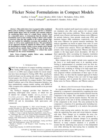
CORAM et al.: FLICKER NOISE FORMULATIONS IN COMPACT MODELS2813Fig. 1. Creation of cyclostationary noise by a periodically varying bias m(t)in a modulated stationary noise model.noise before it reaches the terminals of the component, asshown in Fig. 1.This assumption results in modulated stationary noisemodels [11] that fit very naturally into simulators.1 For example, consider an RF noise analysis like Pnoise. It works verymuch like the traditional noise analysis, except the timevarying operating point modulates both the noise producedby the component and the transfer function from the component to the output. With modulated stationary noise models,the noise from the component is easily partitioned into twopieces: 1) the underlying bias-independent noise, representedby its power spectral density S(f ) and 2) the modulation of thenoise by the component itself, represented by m(t). It is naturaland easy for the simulator to combine the modulation from thecomponent, m(t), with the modulated transfer function of thecircuit, making the overall computation straightforward.Modulated stationary noise models work well for modelingthe flicker noise in linear resistors, which is due to a fluctuationin the value of the resistance over time [12], [13]. The resistoris linear, so this effect is completely independent of bias. Weoften think of the flicker noise of a resistor as being producedby a series voltage source or a shunt current source, but this isan approximation that allows us to think of the resistor as timeinvariant. Consider a resistor that has resistance of R δr(t)where R is the nominal resistance and δr is the fluctuationof the resistance due to flicker noise. Assume the resistor isdriven with a dc current I. Then,V δv(t) (R δr(t)) · I.(1)The resulting noise voltage isδv(t) δr(t) · I(2)which includes a bias-independent flicker noise component,δr, and a bias-dependent modulation term, I.Modulated stationary noise models are not completely general. There are observed circuit behaviors that cannot be modeled using modulated stationary noise sources. For example,1 In this article, we use the term stationary to denote a noise process wherethe statistics do not change with time, meaning that the average value (themean), the power level (the variance) and the correlations (the autocorrelationfunction) are constant. We use the term cyclostationary to refer to a noiseprocess where these quantities do vary with time, but in a cyclic fashion.We use the terms modulated and nonstationary to refer to noise processeswhere the statistics do vary with time, so cyclostationary processes are alsononstationary. In addition, a flicker noise process with a true 1/f power spectral density is nonstationary because the statistical metrics break down as theperiod of observation becomes infinite (the variance, or noise power, increaseswithout bound as f goes to zero). However, real devices cannot behave thatway. The noise flattens out at low frequencies, making their total noise powerfinite [12]. We confine ourselves to real devices and so consider a flicker noiseprocess to be stationary or not-based only on whether it is modulated.the low-frequency noise produced by some circuits can bereduced by regularly switching off the bias of the circuit [10].This effect cannot be accurately modeled using modulatedstationary noise sources. Despite these limitations, modulatedstationary noise models are suitable in many common situations; and when not completely accurate, often provide a goodstarting point that is accurate to first order.Consider flicker noise in MOSFETs. A reasonable firstorder model is to assume that the flicker noise is a biasindependent variation in the value of the threshold voltage, VT .Again, because we like time-invariant models, we model theflicker noise by adding a time-varying current source in parallel with the channel, where the current in this noise sourceis roughly equal to the fluctuation in VT multiplied by thetransconductance of the FET, gm . This is a modulated stationary noise model where m gm and it is the basic approach thathas been used by simulators for many years. While it is notcompletely accurate for switched-bias circuits, it has provenuseful and predictive for a wide variety of other circuits.III. SPICE F LICKER N OISE M ODELIf we assume that a resistor that exhibits flicker noise isdriven with a constant voltage V, thenI δi(t) V.(R δr(t))(3)By recognizing that V IR and rearranging the terms this canbe written asδi(t) I · δr(t)/R.(4)Thus, the power spectral density of the expected noise current isK(5)Sii I 2 Srr I 2 .fThe traditional model used to represent flicker noise of acurrent I in SPICE isKF · I AFSii .(6)f EFSPICE does not model flicker noise for a resistor, but this formis used for the diode, JFET, and MOSFET [4]. This equationmatches (5) if KF K, AF 2, and EF 1.AF and EF are fitting parameters. There is little to no physical justification for them to be different from their defaultvalues of 2 and 1. Nonetheless, they are well established andare routinely set to values different from their defaults.IV. M ODELING F LICKER N OISE IN V ERILOG -AA key benefit of Verilog-A is that many analog simulatorssupport dynamic compilation of user-supplied models writtenin Verilog-A. We are thus able to test out flicker noise models in various simulators without needing to change either thesimulators or their built-in models. A simple linear resistorwith flicker noise is sufficient to produce our key result.In Verilog-A, a resistor of value R between nodes a and bis implemented viaIr V(a,b)/R;I(a,b) Ir;Authorized licensed use limited to: Kenneth Kundert. Downloaded on November 05,2020 at 18:20:48 UTC from IEEE Xplore. Restrictions apply.
2814IEEE TRANSACTIONS ON COMPUTER-AIDED DESIGN OF INTEGRATED CIRCUITS AND SYSTEMS, VOL. 39, NO. 10, OCTOBER 2020The contribution operator adds a current through thebranch connecting the nodes a and b of value Ir. A complete Verilog-A implementation of a resistor can be found inthe Appendix; sample netlists can be downloaded from [14].Noise in the resistor can be contributed as wellI(a,b) white noise(4.0*‘P K* temperature/R, "thermal");where the value of Boltzmann’s constant ‘P K is defined in aheader file provided in the LRM, and temperature is thecircuit analysis temperature in Kelvin. This contribution creates a small-signal noise current source on the branch (a,b)with a frequency independent power spectral density whosevalue is specified by the first argument; the second argumentis a name for the simulator to give when presenting results.Flicker noise for a resistor is usually modeled as being afunction of the dc current Ir through the resistorFig. 2. Pnoise simulation results for a 100 resistor driven by a 0.1 Vamplitude sinusoid at f0 217 Hz. KF 10 6 , AF 2, EF 1.Pn KF*pow(abs(Ir), AF);I(a,b) flicker noise(Pn,EF, "flicker");(7)where KF, AF, and EF are parameters of the model that areadjusted to fit measured data and Pn is the amplitude of thenoise power for f 1. KF is a prefactor; AF is the exponentof the current; and EF is the exponent of frequency, which isexactly 1.0 for true 1/f noise.The deterministic current Ir (dc or transient) may be positive or negative, and while AF is 2 by default, it may be fractional. Trying to compute pow(Ir, AF) results in a matherror if Ir 0 and AF is not an integer. Further, a noise powerspectral density must be non-negative. Hence, most modelsinclude the abs() call in pow(abs(Ir),AF) without further thought. Indeed, the Verilog-AMS LRM itself (Section4.6.4.5 in version 2.4) provides the following expression forflicker noise in a diode:Fig. 3. TRnoise reference simulation results, same device and conditions asFig. 2.flicker noise(kf*pow(abs(I( a )), af), ef)However, this expression is incorrect and gives rise to peculiarresults, as the next section shows.V. S IMULATION R ESULTSIn [12], analysis of a linear resistor driven by a sinusoidalvoltage source of frequency f0 shows that 1/f noise shouldbe a spectrum that varies as 1/ f f0 . Fig. 2 shows Pnoisesimulation results of the model (7) compared to the expectedreference behavior of [12]. HBnoise simulation results are,to within numerical tolerances, the same as the Pnoise results.Figs. 3 and 4 show TRnoise simulation results for the referencemodel and the model (7), respectively; they are consistent withthe Pnoise and HBnoise results.Clearly, the model (7) does not work properly for noiseunder large-signal time-varying conditions when Ir changessign. It incorrectly exhibits a dc-like 1/f component, althoughthere is no dc current, it lacks the expected 1/ f f0 sidebands,and it has components at integer multiples of 2f0 , which shouldnot be there.Fig. 4. TRnoise simulation results using the model (7), same device andconditions as Fig. 2.VI. C OSINE M IXER P OWER S PECTRAL D ENSITYIn this section, we derive the power spectral density foran ideal cosine mixer. We then extend this in Section VII toanalyze the incorrect results from the model (7).The autocorrelation of a random signal x(t) is [15]Rxx (t, t τ ) E[x(t) · x(t τ )](8)where E() denotes expectation. x(t) is cyclostationary withperiod T 1/(2π f0 ) if the autocorrelation is invariant to aAuthorized licensed use limited to: Kenneth Kundert. Downloaded on November 05,2020 at 18:20:48 UTC from IEEE Xplore. Restrictions apply.
CORAM et al.: FLICKER NOISE FORMULATIONS IN COMPACT MODELS2815translation by T, i.e., ifRxx (t, t τ ) Rxx (t T, t τ T).(9)In this case, we can expand Rxx as a Fourier seriesRxx (t, t τ ) Rxk (τ ) · ej2π kf0 t(10)k where the Fourier coefficients, which [7] calls “harmonicautocorrelation functions,” are 1 TRxk (τ ) Rxx (t, t τ ) · e j2π kf0 t dt.(11)T 0The “harmonic power spectral densities” [7] are the Fouriertransforms of these harmonic autocorrelation functions Sxk (f ) Rxk (τ ) · e j2π f τ dτ.(12) Consider a sinusoidal mixer having unity amplitude andfrequency f0 , with input x(t) and output y(t)y(t) cos(2π f0 t) · x(t).(13)If the signal x(t) contains noise we want to determine thepower spectral density of the output signal y(t), which is cyclostationary as long as x(t) is stationary or cyclostationary withperiod 1/f0 . Further, from (8), (10), and (13)Ryy (t, t τ ) E cos(2π f0 t) · x(t) · cos 2π f0 (t τ ) · x(t τ ) cos(2π f0 t) · cos 2π f0 (t τ ) · E[x(t) · x(t τ )] cos(2π f0 t) · cos 2π f0 (t τ ) · Rxx (t, t τ ) cos(2π f0 t) · cos 2π f0 (t τ ) ·Rxk (τ )ej2π kf0 tk (14)so the harmonic autocorrelation functions of y are 1 T Ryi (τ ) cos(2π f0 t) · cos 2π f0 (t τ )T 0 Rxk (τ )ej2π(k i)f0 t dt. Fig. 5.Resistor model that includes modulated flicker noise.where the integration and summation order was changed.Now cos(a) 0.5 · (eja e ja ), so the inner integral overdτ in (16) is ej2π f0 (t τ ) e j2π f0 (t τ ) · e j2π f τ · Rxk (τ ) dτ0.5 j2π f0 t 0.5 · ee j2π (f f0 )τ · Rxk (τ ) dτ 0.5 · e j2π f0 te j2π(f f0 )τ · Rxk (τ ) dτ 0.5 · ej2π f0 t Sxk (f f0 ) 0.5 · e j2π f0 t Sxk (f f0 ).(17)Using this in (16) and replacing cos(2π f0 t) by its complexexponential form gives T 1Syi (f ) 4T 0k Sxk (f f0 ) ej2π(k i 2)f0 t ej2π(k i)f0 t Sxk (f f0 ) ej2π(k i 2)f0 t ej2π(k i)f0 t dt. (18)Because of the periodicity of the complex exponential 1 T j2π kf0 t(m n)edt δm,nT 0(19)where δm,n is the Kronecker delta, only four terms of thesummation in (18) are nonzero, for k i, i 2, soSyi (f ) (15)k The harmonic power spectral densities of y are then T 1Syi (f ) cos(2π f0 t) · cos 2π f0 (t τ ) T 0 Rxk (τ )ej2π(k i)f0 t dt · e j2π f τ dτ 1 Sx (f f0 ) Sxi (f f0 )4 i 2 Sxi (f f0 ) Sxi 2 (f f0 )(20)which is consistent with (3) of [7]. For a stationary input, Sxk isnonzero only for k 0, and we typically measure the averageoutput noise Sy0 , so this becomesSx0 (f f0 ) Sx0 (f f0 ).(21)4This means that the noise spectrum of x(t) is frequency shiftedby the mixer to f0 . This is precisely the behavior of thereference results in Figs. 2 and 3, and it matches the resultsin [12], obtained by a different method.Sy0 (f ) k 1 Tcos(2π f0 t) · ej2π(k i)f0 t T 0k cos 2π f0 (t τ ) · e j2π f τ · Rxk (τ ) dτ dt (16)VII. M ODULATED F LICKER N OISEConsider the circuit in Fig. 5, which has an independentvoltage source v(t) driving a resistor, and a dependent currentsource whose value is the product of current in the resistorand the noise voltage x(t).Authorized licensed use limited to: Kenneth Kundert. Downloaded on November 05,2020 at 18:20:48 UTC from IEEE Xplore. Restrictions apply.
2816IEEE TRANSACTIONS ON COMPUTER-AIDED DESIGN OF INTEGRATED CIRCUITS AND SYSTEMS, VOL. 39, NO. 10, OCTOBER 2020This equivalent circuit is a modulated stationary noise modelthat separates the flicker noise process from the bias dependence in a way that makes the analysis more tractable andbypasses questions about whether the bias dependence affectsthe statistics of the random process [7]. The random processis bias-independent and stationary, and the bias dependence isintroduced by the deterministic modulation. This interpretationaligns with van der Ziel’s description of flicker noise as afluctuation of the resistance and the current as a method ofdetecting it [12]; when the current is time-varying, it modulatesthe observed noise spectrum [see (5)].If v(t) is a dc source, i.e., v(t) V, then the dependent source provides a constant gain of V/R to the noisesource, and the noise current power spectral density is theproduct of (V/R)2 and the power spectral density of x(t).If x(t) is a flicker noise source with power spectral densitySxx (f ) KF/f , then the current noise power spectral density is 2V KF.(22)Sii (f ) RfThis is just (7) with AF 2 and EF 1, and is equivalent tothe result (5) derived from a resistance fluctuation viewpoint.For a dc bias, the absolute value does not matter; the autocorrelation (and hence power spectral density) depends on thesquare of the signal, so the gain is squared, eliminating anyminus sign.If the voltage source is a cosine source, v(t) cos(2π f0 t),the situation changes. When the dependent source multipliesthe noise by the current, we recover the mixer situation analyzed in the previous section, and we get the familiar outputnoise power spectral density, consisting of copies of the 1/fspectrum shifted to f0 .However, if the dependent source multiplies the noise bythe absolute value of the current, so i(t) x(t) · v(t)/R , theanalysis of the previous section breaks down. Equation (16)becomes 1 T cos(2π f0 t) · ej2π(k i)f0 tSyi (f ) T 0k j2π f τ cos 2π f0 (t τ ) · e · Rxk (τ ) dτ dt. (23)To evaluate (23) we need to introduce the Fourier series of cos(2π f0 t) . This is cos(2π f0 t) ak · ej2π f0 kt(24)k where1ak T T cos(2π f0 t) · e j2π f0 kt dt02·( 1)k/2π ·(1 k2 )0for even kfor odd k.(25)Intuitively, if we modulate the noise by cos(2π f0 t) , we wouldexpect a dc component as well as even harmonics, but noFig. 6.Results of Fig. 2 with linear abscissa scale.odd harmonics, and (25) verifies that these are the components selected from (23). This is also precisely the behaviorof the incorrect results in Figs. 2 and 4 from the VerilogA noise model of (7) that uses abs(Ir). Fig. 6 show theresults of Fig. 2 with a linear abscissa scale, which makes thefrequencies of the harmonics more apparent.We note that (16) and (23) are identical when x is whitenoise, uncorrelated in time [Rxx (t, t τ ) δ(τ ), where hereδ(τ ) is the Dirac delta function, which means that Rx0 (t, t τ ) δ(τ ), and the other harmonic autocorrelation functionsRxk (τ ) 0, k 0]. Accounting for the sign of the modulatingsignal is necessary only for colored noise.Consider also the scenario where v(t) is a square wave: if thenoise is determined by the absolute value of the modulation,then this situation would be indistinguishable from a dc bias(other than the short transition times).VIII. E XTRACTING THE M ODULATION F UNCTIONHow did this happen? How did we end up taking the absolute value of the modulating signal? It is easy to say that theproblem is coming from the use of the absolute value functionin (7). While that is certainly true, there is more to it. Considerthe simpler case of where AF is fixed to 2 as in (6)K(26)Sii I 2 .fDecomposing this into a modulatedstationary noise model gives S K/f and m (I 2 ) I . The square root isrequired to convert I 2 from a power. Remember that each positive number has two square roots: 1) one positive and 2) onenegative. In this case, we chose the positive one, but we couldhave easily chosen the negative one. At the time we wereassuming dc conditions, so the sign is irrelevant because mis multiplied by values from a stochastic process with zeromean. However, when the operating point changes with timewe have to be more careful. We can see from (4) that themodulation function is m I, but as before the minus signis irrelevant, so we can use either I. However, if we alwayschoose the positive root for m, even when I changes sign, thisis in effect alternating which root is chosen as a function oftime, which is not permissible. The fundamental problem isthat the amplitude of the flicker noise is specified as a power,which means the sign of the modulation function m is lost.Authorized licensed use limited to: Kenneth Kundert. Downloaded on November 05,2020 at 18:20:48 UTC from IEEE Xplore. Restrictions apply.
CORAM et al.: FLICKER NOISE FORMULATIONS IN COMPACT MODELS2817One way to solve this problem is simply make the noisepower argument of the flicker noise function constant andinstead modulate the output of the function. This is naturalif you know the modulation function. For example, for thissimple case we know m I and so we can model the noisewithI(a,b) -Ir*flicker noise(K,EF, "flicker");(27)However, in many cases, it is easier to work with the noisepower because that is what is readily available, as with (6).That case is considered next.IX. R EVISED V ERILOG -A I MPLEMENTATIONAs described in Section VII, periodic and TRnoise analysesuse the modulated stationary noise model [7]. The noise inputu(t) is expressed as u(t) m(t) · us (t) where m(t) is the modulation and us is stationary noise. The PSD of u, Suu , theninvolves Mi the Fourier coefficients of m(t). Without goinginto the details that be found in [7], we note here that whenSus us is frequency independent (white), the sign of m(t) endsup not being necessary. However, for flicker and colored noisesources, we must preserve information about the sign of m(t).We would like to convey the sign of m(t) to the variousnoise analyses, by choosing an alternative expression whenIr is negative [Pn is defined in (7)]if (Ir 0) beginI(a,b) flicker noise ( Pn,EF, "flicker" );end else begin// alternative expression goes hereendSeveral alternatives appear possible for a Verilog-A model toconvey the sign of m(t) to the various noise analyses// Alternative 1// add minus sign in first argumentI(a,b) flicker noise (-Pn,EF, "flicker" );// Alternative 2// add leading minus signI(a,b) -flicker noise ( Pn,EF, "flicker" );// Alternative 3// swap terminal orderI(b,a) flicker noise ( Pn,EF, "flicker" );For any dc bias condition, we expect all of these implementations to give the same small-signal noise as (7), becauseonly one of the if clauses is active. During a transient analysis or periodic excitation where Ir changes sign, we expectto obtain different noise results. Unfortunately, the results areFig. 7.Pnoise simulation results, alternative noise model implementations 1, 2, and 3, same device and conditions as Fig. 2.not what we want. These three alternatives each describe twonoise sources, one of which is active for positive Ir (and zerofor Ir 0), and the other is active for negative Ir (and zerofor Ir 0). Since their names are the same, the contributionsare combined in the noise summary report, per Section 4.6.4 ofthe Verilog-AMS LRM [1], but the noise sources are independent, and hence uncorrelated. Each noise source is modulatedby a half-wave rectified cosine. The Fourier coefficients forthe component that is nonzero in the first and fourth quartercycles is k/2 for even k π( 1)·(1 k2 )(28)ak 1/4for k 1 0for odd k 1and a similar set of coefficients apply to the component thatis nonzero in the second and third quarter cycles. Besides thedc and even harmonic components, as for the absolute valuemodulation case, (28) indicates there should also be a component at the fundamental frequency f0 . Fig. 7 shows simulationresults from these three alternatives, which are identical; theadditional component at f0 is clear compared to Fig. 6, but theydo not give the correct results (the “reference” curve of Fig. 2).We must instead use one of the following two alternatives,which have only one flicker noise call and hence oneflicker noise source:// Alternative 4// change sign of argumentif (Ir 0) beginPn -Pn;endI(a,b) flicker noise ( Pn,EF, "flicker" );// Alternative 5// add prefactor of /- 1integer sgn;sgn (Ir 0) ? 1 : -1;I(a,b) sgn * flicker noise ( Pn,EF, "flicker" );Authorized licensed use limited to: Kenneth Kundert. Downloaded on November 05,2020 at 18:20:48 UTC from IEEE Xplore. Restrictions apply.
2818IEEE TRANSACTIONS ON COMPUTER-AIDED DESIGN OF INTEGRATED CIRCUITS AND SYSTEMS, VOL. 39, NO. 10, OCTOBER 2020requires an internal node// Alternative 6// use internal nodeelectrical noi;// stationary flicker noiseI(noi) flicker noise(KF, EF,"flicker");// convert noise current to voltageI(noi) V(noi);Fig. 8. Pnoise simulation results, alternative noise model implementation 4or 5, same device and conditions as Fig. 2.// modulate noiseI(a,b) Ir * V(noi);This alternative closely follows (27) and has been tested inseveral commercial simulators. However, it requires an extrainternal node for each flicker noise source.X. OTHER D EVICE M ODELSThe noise power formulation for flicker noise is common,examples from bipolar and diode models include.1) Mextram (version 504.12):powerFBC1fB1 KF M * (1.0-XIBI)* pow((abs(Ib1)/(1.0-XIBI)), AF);I(b2,e1) flicker noise(powerFBC1fB1, 1);Fig. 9. TRnoise simulation results, alternative noise model implementation4 or 5, same device and conditions as Fig. 2.2) HiCuM (version 2.4.0):flicker Pwr kf* pow(abs(ibei ibep),af);I(br biei) flicker noise(It may seem peculiar that the noise power argument Pn inalternative formulation 4 is negative for Ir 0, but the LRMdoes not require the first argument of flicker noise to benon-negative. Allowing negative values for Pn in the integralsof (16), instead of using their absolute values, changes theresults of the integration. In effect, when implemented properly, the simulator is allowing you to choose the root it usesfor m(t) when computing m Pn. If Pn is positive, thepositive root is chosen, if Pn is negative, then the negativeroot is chosen.Alternative 5 is actually a modification of the approachfound in (27), where only the sign ( 1) of the modulationis used as a prefactor.Fig. 8 shows Pnoise simulation results for these two alternatives, which are identical. Clearly, this behavior matches the f0 frequency shifted noise predicted by (21) and the reference results of Fig. 2. TRnoise simulation results-based thesealternative implementations also match those of the referencemodel; compare Figs. 3 and 9. The Appendix contains complete Verilog-A code for a resistor with flicker noise usingAlternative 4.Note that some simulators may not properly simulate oneor the other of these alternatives, as will be discussed inSection XI. There is another alternative formulation, whichflicker Pwr,1.0, "flicker");3) Diode CMC:jfnoise KF i* pow(abs(ijun)*MULT i, AF i);I(A, AIK) flicker noise(jfnoise, 1.0, "flicker");Bipolar and diode currents, and therefore flicker noise, aregenerally negli
flicker noise in Verilog-A compact models, and how a simulator . Kiran K. Gullapalli is with the Design Enablement, Analog and Mixed Signal, NXP Semiconductors, Austin, TX 78735 USA. Kenneth S. Kundert is with Designer’s Guide Consulting