WIXLIB

106E. Fitz-Rodríguez et al. / Computers and Electronics in Agriculture 70 (2010) 105–116The “optimum” environmental conditions have been heuristically determined and defined by growers and researchers throughmany years of experimentation, and today these optimum conditions are successfully achieved by implementing crop-specificblueprints for the manipulation of several actuators (exhaust fans,ventilation openings, shade curtains, heaters, boilers, water pumps,etc.) with simple ON–OFF control to reach desired set-points.However, with the advancements of computer technologies it hasbecome possible to monitor and control several parameters, andto implement more sophisticated control strategies that are basedon modern control theories. These control schemes depend onmathematical models, describing the dynamics of the coupledcrop-greenhouse system, to adjust set-points dynamically to optimize crop growth for a given performance criterion (Seginer, 1993;van Straten et al., 2000).As summarized by von Zabeltitz (1999) several greenhousemodels, based on energy and mass balance equations, have beeninvestigated in the past and they can be classified as static ordynamic models. The more complex models are coupled with thecrop dynamics (e.g., Jones et al., 1988, 1990; Takakura et al., 1971),and they include several state variables describing the status ofthe system over time. Some models address specific phenomena,for example natural ventilation (e.g., Al-Helal, 1998; Boulard andDraoui, 1995; Boulard et al., 1999; Dayan et al., 2004; de Jong,1990), forced ventilation (e.g., Arbel et al., 2003; Willits, 2003),evaporative cooling (e.g., Abdel-Ghany and Kozai, 2006; Baille etal., 1994; Boulard and Baille, 1993; Boulard and Wang, 2000), orheating systems (e.g., Bartzanas et al., 2005; Kempkes et al., 2000).Newer research approaches for greenhouse climate control arebased on an optimization principle, for example for reduced energy(e.g., Aaslyng et al., 2003; de Zwart, 1996; Körner, 2003), andwater consumption (e.g., Blasco et al., 2007); for optimizing CO2usage (e.g., Jones et al., 1989; Linker et al., 1998; Seginer et al.,1986), or humidity control (e.g., Daskalov et al., 2006; Jolliet, 1994;Korner and Challa, 2003; Stanghellini, 1992). Other climate control schemes implement different type of control criteria suchas economic-based optimal control (e.g., Tap, 2000; van Henten,1994), adaptive control (e.g., Udink ten Cate, 1983), multi-objectivehierarchical control (Ramirez-Arias, 2005), or nonlinear predictivecontrol (e.g., El-Ghoumari, 2003). All these approaches offer theadvantage of making efficient use of the resource in study, by maximizing the production return or minimizing the production cost,over the traditional greenhouse control strategies where the setpoints are defined by the grower experience.Greenhouse production systems have a complex dynamicdriven by external factors (weather), control mechanisms (ventilation openings, exhaust fans, heaters, evaporative cooling systems,etc.), and internal factors (crop and internal components). Thusthe more we understand the physics of the greenhouse environment, the better the greenhouse design and component selectionthat will improve the possibilities for success. Several efforts havebeen completed to increase the understanding of greenhouse cropproduction systems through the development of educational materials available on the Internet. Some of these efforts allow foraccess to interactive digital media describing most of the U.S.greenhouse industry (Tignor et al., 2005, 2006, 2007), to living laboratories through web-based monitoring systems that enhancedan asynchronous education by allowing students to monitor current and historical conditions of experimental greenhouse cropsat different off-campus locations including one at the South Pole(Fitz-Rodriguez et al., 2003), to virtual labs with emphasis on control theory applied to greenhouse climate control (Guzmán et al.,2005b), or to a scale-down greenhouse model for remote testcontrol strategies (Guzmán et al., 2005a). While the latter two interactive tools allow for remote access and control, they are tied to onespecific greenhouse configuration design.Several sophisticated and more complete greenhouse environment models currently exist, however they are too complicatedto be implemented into a generic model to predict the behaviorof a wide range of greenhouse designs and climate conditions.The current simplified greenhouse environment model, based onenergy and mass balance equations follows the models proposedby Takakura (1976), and Takakura and Fang (2002).The objective of the current project was to investigate andimplement a dynamic greenhouse environment model describing the dynamic behavior of the greenhouse environment (insideglobal radiation, air temperature, and air moisture content) duringa 28-h interval, which was applicable to different, user-selectablegreenhouse design configurations and geographic locations, yetsimple enough to be implemented in a web-based interactiveapplication for educational purposes. The greenhouse environment dynamics is a complex phenomenon. It is not the objectiveof the current research to fully develop a model for detail andaccuracy, but to simulate realistic environmental responses foreducational purposes by demonstrating the fundamental dynamicsof the greenhouse environment.2. Materials and methodsThis project was developed as part of a multi-institutional(The University of Vermont, University of Florida, The OhioState University, and The University of Arizona) collaborativeeffort to develop web-based educational materials for worldwidegreenhouse education (http://www.uvm.edu/wge/). The projectincluded the development of: (1) digital videos describing thegreenhouse production systems at each location, (2) a searchablerepository of greenhouse educational materials including images,videos and software, (3) a web-based student evaluation methodto determine the extent of learned greenhouse concepts, and (4)a greenhouse environment simulator (Tignor et al., 2006, 2007).The greenhouse environment simulator is a computer simulationprogram based on a greenhouse environment mathematical modeland was programmed in ActionScript 2.0, and integrated into aninteractive interface developed in Flash MX (Flash MX Pro 2004,Macromedia, San Francisco) (Fitz-Rodriguez, 2006). The components of the simulation program included climate data, a databaseof the greenhouse structure and hardware equipment features, andthe mathematical model representing the physics of the greenhouse and crop environment.2.1. Climate dataClimate data from the geographic locations representing eachof the four universities were used to provide the outside environmental conditions as inputs to the simulations. Summarizedby von Zabeltitz (1999) the two climate parameters defining theclimate control strategies and crop production cycles are averagedaily insolation, and average daily air temperature. These are documented for the four sites in Fig. 1. Although in all four locations thelimit of daily radiation (7.4 mol m 2 d 1 ) (3.6 MJ m 2 d 1 ) for effective production is exceeded, only Arizona and Florida have dailyradiations above the minimum required for feasible winter production (17.1 mol m 2 d 1 ). Vermont and Ohio will require artificiallighting for winter production. The daily average air temperature(Tout24 ) defines the type of climate control required. In this way,for the months of April through October when average air temperature is between 12 and 22 C natural ventilation is enough tocontrol the greenhouse environment for Vermont and Ohio. Forany other month when Tout24 12 C a heating system is required.In contrast, the average air temperatures in Florida are above thethreshold value (Tout24 22 C) defined as the need for an artificial

E. Fitz-Rodríguez et al. / Computers and Electronics in Agriculture 70 (2010) 105–116107Fig. 1. Average photosynthetic photon flux (PPF) versus average daily air temperature for every month of the year for each location. Data source from NASA SurfaceMeteorology and Solar Energy: SolarSizer Data (http://eosweb.larc.nasa.gov/).cooling system for most of the year. Arizona has the three situations, during the winter it requires heating, climate control onlywith natural ventilation is possible for several months, and duringthe summer an artificial cooling system is required. All four sitesprovided a wide range of possibilities to simulate the greenhouseenvironment during several production seasons.2.2. Greenhouse structure and componentsGreenhouse structures are designed to overcome the adversities of external (wind, rain, snow, etc.) environmental factors, andinternal (live and dead) loads, while maximizing the solar radiation available for the crop. The greenhouse structural componentsand their geometry directly affect solar radiation transmission.The shape and size of the three greenhouse structural designs(Fig. 2) used in the simulations include: (1) A-frame, (2) Arch-roofand (3) Quonset style, that are some of the most widely used insmall production systems. The geometry of the greenhouse designsimplemented in the simulations is indicated in Table 1. The lengthof each was assumed as 30 m, while the widths were 10, 10 and 8,respectively.The glazing material used in the simulations included singlelayer (glass, polyethylene film, and polycarbonate) and double layerTable 1Dimensions and properties of greenhouse designs used in the simulations.PropertyA-frameArch-roofQuonsetLength (m)Width (m)Gutter high (m)Ridge high (m)Afl (m2 )Agl (m2 )Volume (m3 )w ratio (Agl /Afl 2404277451.8(polyethylene film and polycarbonate) glazing. Their material properties are summarized in Table 2. Internal shade curtains wereoptional in the simulator and included effective shading values of30, 50, and 70% reduction of outside solar radiation in addition tothe reduction caused by the glazing material.Although there are many types and sizes of heating systems ingreenhouses such as steam, hot water, hot air and infrared radiation, only a hot air system was selectable. Heaters, with a capacityof 75 kW each, could be included in the simulation with 1 or 2 ornone as possibilities.The reduced air movement and air exchange within the greenhouse, imposed by the glazing material, results in a greater airtemperature than outside. The greenhouse air temperature couldbe reduced with either natural or forced ventilation as selectedby the user. Ventilation is a highly complex phenomenon andit was not the objective of the current research to rigorouslymodel it. It was assumed that each simulated greenhouse environment had a ventilation rate equivalent to 2, 10, 20, 30, 60and 120 air changes per hour (AC h 1 ). The ventilation rates foreach greenhouse design are slightly different, because of the differences in greenhouse volumes. Corresponding values are shownin Table 3.Table 2Properties of the greenhouse glazing materials used in the simulations.LayersGreenhouse glazingk-Valuea(W m 2 C 1 )Lighttransmissivityb en from ASAE (2003).Taken from Hanan (1998).

108E. Fitz-Rodríguez et al. / Computers and Electronics in Agriculture 70 (2010) 105–116Fig. 2. Structural designs implemented in the greenhouse environment simulator. All three designs have 30 m of length, and are singlespan. Units are in meters.Table 3Ventilation rates (m3 m 2 s 1 ) implemented with the simulation for each greenhouse structural design.Air exchanges per hour (h 1 )Ventilation rate (m3 m 2 s 1 020.0090.0180.0260.0520.1052.3. Mathematical modelThe mathematical model described the state of the greenhouseenvironment and consisted of a system of three first-order differential equations which were derived from energy and massbalance principles. The parameters described by the state equationsinclude: (1) Tin , air temperature ( C), (2) Win , absolute humidity(gwater kg 1) and (3) Tf , ground surface temperature ( C).dry air2.3.1. Energy balance equationEnergy balance equations can be derived under steady-stateconditions for the thermal interaction of each of the greenhousecomponents. von Zabeltitz (1999) described the energy balanceequations of four interacting components (air, plants, floor androof) to define the resulting greenhouse environment. Fig. 3 contains a depiction of the energy and mass fluxes of a ventilatedgreenhouse. A simplified and augmented energy balance equationto describe the greenhouse environment can be expressed as (ASAE,2003):QGRin QHeater QIV QGlazing(1)where QGRin is the global radiation absorbed within the greenhouse(W m 2 ), QHeater is the thermal energy provided by the heatingsystem (W m 2 ), QIV is the energy exchange by infiltration andventilation (W m 2 ) and QGlazing is the heat loss through the glazing (W m 2 ). In the present project, we assumed that the net longwave radiation emitted or stored by plants, structure and glazingwas negligible, as the magnitude of the radiation emitted by each ofthese components is of the same order and they cancel each other.The global radiation absorbed inside the greenhouse QGRin wasestimated with the following equation:QGRin c · (1 g ) · QGRout(2)where c is the solar radiation transmittance of the glazing material(dimensionless), g is the reflectance of the solar radiation on theground surface (dimensionless), and QGRout is the outside globalradiation (W m2 ).The heat lost due to ventilation and infiltration (QIV ) was computed with the following equation:QIV L · E qv · Cp · · (Tin Tout )(3)The two components in the right side of Eq. (3) define the latentand sensible heat losses, respectively, where L is the latent heatof vaporization of water (J kg 1 ), E is the evapotranspiration ratewithin the greenhouse (kg m 2 s 1 ), qv is the ventilation rate(m3 m 2 s 1 ), Cp is the specific heat of moist air (J kg 1 K 1 ), isthe specific mass of air (kgdry air m 3 ), and (Tin Tout ) defines theair temperature difference, between inside and outside the greenhouse, respectively.The heat flux lost through the glazing (QGlazing ) was calculatedwith the following equation:QGlazing k · w · (Tin Tout )(4)where k is the overall heat transfer coefficient (W m 2 C 1 ) and wis a ratio (dimensionless) of the glazing (Agl ) to ground (Afl ) surfaces.The thermal radiation provided by the heating system (hot air)was defined by a constant function depending on the number ofheaters (NH ) of predefined capacity (Hcap ) and expressed per unitground surface (Afl ) asQHeater NHFig. 3. Energy and water vapor fluxes within the greenhouse which define theenergy and mass balance equations. See Table of Nomenclature for definitions ofeach parameter and variable.HcapAfl(5)2.3.2. Mass (water vapor) balance equationFor the mass balance of the air within the greenhouse it wasassumed that no condensation occurred on the inside surface ofthe glazing, no evaporation resulted from the ground surface, andthat the only sources of water to the greenhouse aerial environment was introduced by the evaporative cooling system (EC ) or by

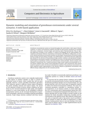
E. Fitz-Rodríguez et al. / Computers and Electronics in Agriculture 70 (2010) 105–116transpiration from the plants (ET ). The only water loss from the system was due to ventilation (EV ). Then, the mass balance equationwasEC ET EVWin · qv · Wout · qv · E(7)where Win and Wout were the absolute humidity of the air(gwater kg 1), inside and outside the greenhouse, respectively,dry airand E was the evapotranspiration (combined from plants and cooling system) rate (kg m 2 s 1 ) within the greenhouse.There are several evapotranspiration models for greenhousecrops reported in the literature and most of them include factorssuch as vapor pressure deficit (VPD), leaf temperature and windspeed. As described by Jolliet (1999), the factor that showed thehighest correlation with transpiration was the inside solar radiation. It was assumed that transpiration was a linear function of thesolar radiation within the greenhouse. The maximum transpiration rate ET 8.9 kg m 2 d 1 taken as a reference, corresponded tosummer conditions in Tucson, AZ (Sabeh et al., 2006), as this wasthe location with the highest average daily insolation (Fig. 1). Solarradiation was normalized and integrated to the maximum ET of reference. Crop transpiration at 15 min intervals was calculated withthe following regressed equation: ET 0.0003 · c · QGRout 0.00210.00006 · c · QGRout 0.00040for large cropfor small cropfor no crop(8)Considering the greenhouse environment (air enclosed by thegreenhouse glazing) as the control volume with homogeneousproperties of air temperature and absolute humidity within itsentire space, the system behavior could be described by the following first-order differential equations (Takakura and Fang, 2002;Takakura and Son, 2004):1dTin QHeater L · E (Tin Tout ) (QCp · · H GRindt (qv · Cp · w · k))dWin1 · (E (Win Wout ) · qv · )H· dt(9)(10) dTfQ14· · GRin εf · (εa · aTin aTf4 ) hs (Tin Tf ) Cs · Z01000dt ks (Tbl Tf ) · 2Z0 Z1 (11)where Cp is the specific heat of air (J kg 1 K 1 ), H is the averagegreenhouse height (m), and Tf is the temperature of the greenhouseground ( C). Other coefficient definitions and values can be foundin the Nomenclature section.2.3.3. Numerical solutionThe model, consisting of a system of three first-order differentialequations (Eqs. (9)–(11)), was solved numerically using a classical fourth-order Runge–Kutta method as described by Chapra andCanale (2002):yi 1 yi 1(k1 2k2 2k3 k4 )6k1 f (xi , yi )Table 4Input and output parameters in the greenhouse environment model.(6)Considering the two sources of water as one component(E EC ET ), and expressing the water content within the greenhouse air as absolute humidity (gwater kg 1), then the resultingdry airmass balance equation QGRoutsW m 2Tout RHoutk3 f UnitsWoutgwater kg 1dry airWsoutgwater kg 1dry air%VPDoutkPaTin QGRinWsinWingwater kg 1dry airW m 2gwater kg 1dry airRHin%VPDinkPa Tfk2 fDerivedvariablesCCC xi 11h, yi k1 h22(14)xi 11h, yi k2 h22(15)k4 f (xi h, yi k3 h) (16)where yi is the set of state variables in the model and h is the timestep for evaluating the new yi 1 values for each equation. Data usedin the simulations were at 900 s intervals, and h is adjusted from 7to 112 s values to accommodate for different simulation scenarios.Data was interpolated to get intermediate values.2.3.4. Initial conditionsThe numerical solution of the differential equations of the greenhouse model required a set of initial conditions for each of the statevariables, and for time t 0, these were assumed to be Tin Tout ,Win Wout , and Tf Tin , as provided within the climate data setsfrom each geographic location. Other variables not time-dependentwere calculated directly. These variables included: (1) global radiation inside the greenhouse (QGRin ), which was a function of thestructure, glazing and/or shade curtains selected; (2) transpirationfrom plants (ET ), which was defined as a linear function of globalradiation; (3) evaporation (EC ) from the cooling system, defined asa constant function when a cooling control function was selected.A set of input/output variables used in the simulation are listed inTable 4.2.3.5. Control functionsThe resulting greenhouse environment for a specific scenariodepended not only on the external factors (climate), and theresponse of the inside conditions, but also on the control strategiesimplemented. Control strategies included reducing the greenhouseair temperature by using shade curtains, by ventilation or by evaporative cooling, or increasing the air temperature with heaters orby reducing the ventilation rate.The simulation of the greenhouse environment was implemented for two general scenarios: (1) uncontrolled, where initialgreenhouse configurations were selected and the control function of the actuators (shade curtains, ventilation, cooling system,and heaters) were inactivated; (2) controlled, where set-pointsfor air temperature (TspD 24 and TspN 18 C for day and night,respectively) were implemented and the control function for eachcomponent was defined with simple if-then rules to define the status (ON or OFF) for each component. The values for each of thecontrol components for the ON and OFF conditions are listed onTable 5. For the ON condition, there were three levels of shade,five levels of ventilation, two levels of cooling, three levels of plantsizes, and two levels of heating. All OFF conditions were zero,except for Ventilation that was 2 AC h 1 representing infiltrationrate.The control logic for the shade curtains was defined as ifQGRout QGRsp , then shades ON, else OFF, where QGRsp , was the

110E. Fitz-Rodríguez et al. / Computers and Electronics in Agriculture 70 (2010) 105–116Table 5Values for the ON-OFF condition for each of the control components for modifyingthe greenhouse environment.ComponentUnitsStatusONShade curtainsPercent of Shades (%)Ventilation rate(Natural or Forced)Air exchanges N (h 1 )Cooling systemEc (kg m 2 d 1 )aHeating SystemaHcap (kW)OFF30507001020306012027.414.87515000Values taken from Sabeh et al. (2006).threshold value for outside solar radiation, and was equal to800 W m 2 .The greenhouse air temperature was controlled by ventilation,evaporative cooling or by heating, depending whether the inside airtemperature was greater or less than the air temperature set-point.For each case there were two conditions, depending on whether theair temperature was higher (Tin Tsp ) or lower (Tin Tsp ) than theset-points. In each situation the corresponding logic values wereassigned to activate or de-activate the ventilation, the evaporativecooling or the heating systems accordingly.3. Results and discussionThe greenhouse environment model was implemented in aninteractive online web-based application (http://ag.arizona.edu/ceac/wge/simulator/) that incorporated user-selected information from a database of greenhouse designs, operations, andgeographic climate conditions, and which graphically displayeddynamic changes in the greenhouse environment. This computersimulation program allowed users to simulate changes in thegreenhouse–plant environment based on climate, structure, andenvironmental control choices (Fig. 4).The numerical solution provided a dynamic response of thegreenhouse climate to the outside climate conditions and for a particular greenhouse design. The design incorporated user-selectedinputs for climate, structure, glazing, and environmental controlsystems. Each simulation demonstrated the response of a greenhouse system design over a 28-h period.For the amount of user-selectable choices provided by thegreenhouse environment simulator, there were 311,040 possiblescenarios that could be demonstrated. The following greenhouseenvironment simulations were analyzed to show the potential ofthe simulator as an educational tool for demonstrating the physicsof greenhouse systems and environmental control principles.Although the results of the simulated scenarios were not validated with experimental measurements, they were verified withthe logical responses obtained with the control strategies and thesystem implemented. As an educational tool the simulator allowsfor many scenarios that could be compared side-by-side enhancingthe learning experience.3.1. Greenhouse environment simulation with ventilationIn Fig. 5 and Table 6 the results of several simulated ventilation and cooling scenarios are displayed, showing the effect ofreduced air movement within a greenhouse. The environment ofan empty greenhouse (A-frame covered with glass) was simulatedfor the summer conditions at each of the four locations, and fordifferent ventilation rates (for N 2, 10, 20, 30, 60 and 120). Thelargest air temperature condition occurred when there was no airexchange (N 2, air exchange due only to infiltration). Greenhouseair temperatures reached a maximum of between 35 and 40 C inColumbus, OH, between 40 and 45 C in Burlington, VT, and equalto or higher than 50 C in Tucson, AZ and Fort Pierce, FL. By increasing the ventilation rate capacity, the greenhouse air temperaturewas reduced to nearly the outside conditions, which was still unfavorable ( 35 C) for growing plants. Therefore an artificial coolingmechanism was needed during the summer season, to maintainthe desired greenhouse air temperature (24 and 18 C for day andnight time, respectively).3.2. Greenhouse environment simulation with evaporativecoolingIn the previous simulations it was demonstrated that artificial cooling, such as evaporative cooling system

The greenhouse environment simulator was designed to be used as an educational tool for demonstrat-ing the physics of greenhouse systems and environmental control principles. Several scenarios were simulated to demonstrate how a specific greenhouse