Transcription
Advanced Data Mining with WekaClass 3 – Lesson 1LibSVM and LibLINEARIan WittenDepartment of Computer ScienceUniversity of WaikatoNew Zealandweka.waikato.ac.nz
Lesson 3.1: LibSVM and LibLINEARClass 1 Time series forecastingLesson 3.1 LibSVM and LibLINEARClass 2 Data stream miningin Weka and MOAClass 3 Interfacing to R and other datamining packagesClass 4 Distributed processing withApache SparkLesson 3.2 Setting up R with WekaLesson 3.3 Using R to plot dataLesson 3.4 Using R to run a classifierLesson 3.5 Using R to preprocess dataClass 5 Scripting Weka in PythonLesson 3.6 Application:Functional MRI Neuroimaging data
LibSVM and LibLINEARInstall the packages LibSVM and LibLINEAR (also install gridSearch) Written by the same people (National Taiwan University) LibSVM and LibLINEAR widely used outside Weka Weka’s most popular packages!Support Vector Machines Both packages implement them– Weka already has SMO (Data Mining with Weka Lesson 4.5)– . but LibSVM is more flexible; LibLINEAR can be much faster SVMs can be linear or non-linear: “kernel” functions SVMs can do classification or regression– Weka already has SMOreg for regression gridSearch will be used to optimize parameters for SVMs
LibSVM and LibLINEARSMO/SMOreg LibSVM LibLINEARLinear SVM?yesyesyesNon-linear kernels?yesyesno1-class classification?noyesno. two-class classification when there are no negative examplesLogistic regression?nonoyes. Logistic classifier (Data Mining with Weka Lesson 4.4)Very fast?nonoyes!L1 norm?nonoyes. minimize sum of absolute values, not sum of squares
LibSVM and LibLINEARLibLINEARSpeed test Data generator: 10,000 instances of LED24 data, percentage split evaluation– LibLinear2 secs to build model– LibSVM, default parameters (RBF kernel) 18 secschoose linear kernel10 sec– SMO, default parameters (linear)21 secs
LibSVM and LibLINEARLinear boundary small margin 0 errors on training data
LibSVM and LibLINEARLinear boundary small margin 0 errors on training data 4 errors on test data
LibSVM and LibLINEARLinear boundary small margin 0 errors on training data 4 errors on test data
LibSVM and LibLINEARLinear boundary small margin
LibSVM and LibLINEARLinear boundary large margin 1 error on training data
LibSVM and LibLINEARLinear boundary small margin 1 error on training data 0 errors on test data
LibSVM and LibLINEARLinear boundary LibLINEAR LibSVM with linear kernel(or SMO) 21 errorson the training set
LibSVM and LibLINEARNonlinear boundary LibSVM, RBF kerneldefault parameterscost 1, gamma 0 9 errors on training setDo it! with BoundaryVisualizer in Explorer
LibSVM and LibLINEARNonlinear boundary LibSVM:OK parameterscost 10, gamma 0 0 errors on training set Poor generalization
LibSVM and LibLINEARNonlinear boundary LibSVMoptimized parameterscost 1000, gamma 10 0 errors on training set Good generalization
LibSVM and LibLINEAROptimizing LibSVM parameterswith gridSearch
LibSVM and LibLINEAR10ifrom 103gridSearch defaultsdown to 10–3steps of 1C: 103, 102, 10, 1, 10–1, 10–2, 10–3kernel.gamma: 103, 102, 10, 1, 10–1, 10–2, 10–310ifrom 103down to 10–3use SMOreg (regression)steps of 1evaluate using correlation coefficient
LibSVM and LibLINEAR10ifrom 103Optimizing LibSVM parameterswith gridSearchdown to 10–3costLibSVM: parameters cost, gammasteps of 1cost: 103, 102, 10, 1, 10–1, 10–2, 10–310gamma:103,102,10, 1,10–1,10–2,ifrom 10310–3down to 10–3use LibSVM (classification)gammasteps of 1evaluate using AccuracyLibSVM cost 1000, gamma 10Accuracy
LibSVM and LibLINEAR10SMOOptimizing LibSVM parameterswith gridSearchifrom 103down to 10–3c(RBFKernel): c, kernel.gammasteps of 1c: 103, 102, 10, 1, 10–1, 10–2, 10–310kernel.gamma:103,102,10, 1,10–1,10–2,ifrom 10310–3down to 10–3kernel.gammause SMO (classification)steps of 1SMOevaluate using AccuracyAccuracy
LibSVM and LibLINEAR LibLINEAR: all things linear– linear SVMs– logistic regression– can use “L1 norm” minimize sum of absolute values, not sum of squares LibSVM: all things SVM Practical advice for using SVMs:– first use a linear SVM– then select RBF kernel. and optimize cost, gamma using gridSearchReference: Hsu, Chang and Lin (2010) “A practical guide to support vectorclassification” http://www.csie.ntu.edu.tw/ cjlin/papers/guide/guide.pdf
Advanced Data Mining with WekaClass 3 – Lesson 2Setting up R with WekaEibe FrankDepartment of Computer ScienceUniversity of WaikatoNew Zealandweka.waikato.ac.nz
Lesson 3.2: Setting up R with WekaClass 1 Time series forecastingLesson 3.1 LibSVM and LibLINEARClass 2 Data stream miningin Weka and MOAClass 3 Interfacing to R and other datamining packagesClass 4 Distributed processing withApache SparkLesson 3.2 Setting up R with WekaLesson 3.3 Using R to plot dataLesson 3.4 Using R to run a classifierLesson 3.5 Using R to preprocess dataClass 5 Scripting Weka in PythonLesson 3.6 Application:Functional MRI Neuroimaging data
Setting up R with Weka The instructions are based on using 64-bit Windows, 64-bit Java, and 64-bitR, and assume admin rights– Mixing 32-bit versions with 64-bit ones will produce problems, e.g., the installationprocess for Weka’s RPlugin may halt for no apparent reason– If you have 32-bit Windows, use 32-bit Java and 32-bit R– Support for R in Weka can also be installed on OS X and Linux: refer to the installationinstructions that come with Weka’s RPlugin There are four main steps to the installation process:––––Downloading and installing RInstalling the rJava package in RSetting up some Windows environment variablesDownloading and installing the RPlugin package for Weka
Downloading and installing R Choose a download mirror fromhttps://cran.r-project.org/mirrors.html Choose to download the binary distribution for WindowsChoose the “base” version of the distributionOnce downloaded, execute the installerAccept all default settings for install options, but untick 32-bit files whenasked to choose R components to install– If you are using 32-bit Windows, untick 64-bit files instead
Installing the rJava package in R Start the R console, e.g., by double-clicking on the shortcut that the installerhas put on your desktop In the R console, type install.packages("rJava") and press the return key onyour keyboard Note that this will only work if you have direct web access, i.e., if your webaccess is not provided by a proxy computer(see the next slide on what to do if you are behind a proxy) In the pop-up menu, choose a mirror to download from Accept defaults when asked for install options Close R once the package has been installed, by typing q(), without saving theworkspace
For users with web connections provided by a proxy If your organization uses a proxy computer, you need to set up someWindows environment variables before starting R Using the Windows search functionality, search for variables, and select Editenvironment variables for your account Use the New. button to add two new variables, with names HTTP PROXYand HTTPS PROXY Set their value to the URL and port number of your organisation's proxyserver, separated by a comma– For example, at Waikato, this would be http://proxy.waikato.ac.nz:8080 Then, when you install a package in R, you will be asked for your proxy username and password
Setting up the environment variables We need to set up some environment variables so that Weka’s RPlugin knowswhere R and its libraries are located Using the Windows search functionality, search for variables, and select Editenvironment variables for your account Use the New. button to add two new variables, with names R HOME andR LIBS USER (see screenshot on next slide) Set the value of R HOME to the path of the folder containing the R software(it should end in something like R-X.X.X) Set the value of R LIBS USER to the path of the folder containing the newlyinstalled rJava package for R Also, use the Edit. button to add the path of the folder containing the Rexecutable to the PATH variable (after adding a semicolon)– If there is no PATH variable, make a new one
Screenshot of environment variablesMake sure youdon’t use quotesin the variablevalues.In this example, there wasno pre-existing PATHvariable, so the location ofthe R executable is the onlyvalue of the PATH variable.
Installing the RPlugin for Weka Start Weka, and from the Tools menu in the GUIChooser, select the Wekapackage manager Choose RPlugin from the list of packages and press Install– If your internet access is through a proxy server, see Using a HTTP proxy athttp://weka.wikispaces.com/How do I use the package manager– for information on how to configure Weka to use the proxy server In the pop-up dialogues, press OK Once the plugin has been installed, restart Weka Start the Weka Explorer, load the iris data, go to the new RConsole tab, andtype plot(rdata) Once you have pressed return, the iris data will be plotted
What can possibly go wrong? Many things , too many to cover here! If you run into problems with the installation process, don’t despair, just getin touch with the Weka community for help
Advanced Data Mining with WekaClass 3 – Lesson 3Using R to plot dataEibe FrankDepartment of Computer ScienceUniversity of WaikatoNew Zealandweka.waikato.ac.nz
Lesson 3.3: Using R to plot dataClass 1 Time series forecastingLesson 3.1 LibSVM and LibLINEARClass 2 Data stream miningin Weka and MOAClass 3 Interfacing to R and other datamining packagesClass 4 Distributed processing withApache SparkLesson 3.2 Setting up R with WekaLesson 3.3 Using R to plot dataLesson 3.4 Using R to run a classifierLesson 3.5 Using R to preprocess dataClass 5 Scripting Weka in PythonLesson 3.6 Application:Functional MRI Neuroimaging data
First steps with ggplot2 We need some data to work with, so first load the Iris data into thePreprocess panel of the Explorer To plot data with R, go to the RConsole Before we can use ggplot2, we need to download and install thecorresponding R package:– To install the package, type install.packages("ggplot2") and press return– To load the package, type library(ggplot2) and press return Try entering the following to see if the package works:ggplot(rdata, aes(x petallength)) geom density() This should give you a kernel density estimate for the petal length of the Irisflowers
The data layer The first layer is the data layer, which specifies the data we want to plotThe data layer is specified using the ggplot() functionThe first argument of this function is the data we want to plotWe use rdata here, because this is the name of the data that has beentransferred into R from the Preprocess panel The second argument is often a call to the aes() function, which maps datato a plot’s visual aspects and components We use it to define which attributes are plotted, and how parts of the plotare colored and filled
The geometry layer(s) Once the data layer has been defined, we can define geometry layers tospecify how the data is plotted In the previous example, we specified a kernel density plot by using thegeom density() function– The kernel density estimate generated this way is too wide, but we can use the xlim()function to change the range of the x axis:ggplot(rdata, aes(x petallength)) geom density() xlim(0,8) We can use the adjust parameter to scale the kernel bandwidth that is usedby the estimateggplot(rdata, aes(x petallength)) geom density(adjust 0.5) xlim(0,8) Using values smaller than 1 makes the density estimate fit the data moreclosely and we get more peaks and valleys
Plotting classification data In classification problems, we often want to visualize data on a per-classbasis to detect discriminative information We can do that quite easily with ggplot2, e.g., by plotting separate colorcoded estimates for each class value:ggplot(rdata, aes(x petallength, color class)) geom density(adjust 0.5) xlim(0,8) We can also fill the area under the plots based on class color:ggplot(rdata, aes(x petallength, color class, fill class)) geom density(adjust 0.5) xlim(0,8) We can specify the level of transparency by using the alpha parameter as ageometry-specific aesthetic:ggplot(rdata, aes(x petallength, color class, fill class)) geom density(adjust 0.5,alpha 0.5) xlim(0,8)
Generating multiple separate plots (“facets”) We can use facets to display multiple per-attribute plots Generated data has three attributes: class, variable, value First, we need to load the reshape2 library, which has been installed with theggplot2 library:library(reshape2) Then, we use the melt() function to transform the data:ndata melt(rdata) To plot a facet grid, with one row facet per attribute:ggplot(ndata, aes(x value, color class, fill class)) geom density(adjust 0.5, alpha 0.5) xlim(0,8) facet grid(variable .) We can also use column facets:ggplot(ndata, aes(x value, color class, fill class)) geom density(adjust 0.5, alpha 0.5) xlim(0,8) facet grid(. variable)
Printing a plot into a PDF Use pdf() function to redirect output of plot from screen to a PDF file, e.g.:pdf("/Users/eibe/Documents/Test.pdf") Reissue command, so that plot is written to the file:ggplot(ndata, aes(x value, color class, fill class)) geom density(adjust 0.5, alpha 0.5) xlim(0,8) facet grid(. variable) Once the data has been plotted to the file, redirect output back to screen:dev.off() The resulting PDF can be viewed with any PDF reader and integrated intoother documents
One more example of a geometry layer: box plots Assuming we have generated ndata using the melt() function as before, wecan plot box plots for each attribute:ggplot(ndata, aes(y value, x class, color class)) geom boxplot() facet grid(. variable) This will generate four column facets containing box plots, with one box plotper class value in each facet The latter is achieved by using the nominal attribute class as the columnattribute for each facet’s box plot The color is also based on the class, so that columns and colors match foreach box plot
Further information There is a very comprehensive web site with documentation for ggplot2:http://ggplot2.org/ This site also enables you to subscribe to a mailing list where you can gethelp There are several books dedicated to ggplot2, including two that arementioned at the above location
Advanced Data Mining with WekaClass 3 – Lesson 4Using R to run a classifierEibe FrankDepartment of Computer ScienceUniversity of WaikatoNew Zealandweka.waikato.ac.nz
Lesson 3.4: Using R to run a classifierClass 1 Time series forecastingLesson 3.1 LibSVM and LibLINEARClass 2 Data stream miningin Weka and MOAClass 3 Interfacing to R and other datamining packagesClass 4 Distributed processing withApache SparkLesson 3.2 Setting up R with WekaLesson 3.3 Using R to plot dataLesson 3.4 Using R to run a classifierLesson 3.5 Using R to preprocess dataClass 5 Scripting Weka in PythonLesson 3.6 Application:Functional MRI Neuroimaging data
Using supervised learning algorithms from R in Weka R has a large collection of libraries with supervised learning algorithms forregression and classification The MLR package for R provides a unified interface to many of thesealgorithms Weka’s RPlugin contains MLRClassifier, which provides access to theregression and classification schemes in MLR In this way, the regression and classification schemes in MLR can be used likeany other classifier in Weka– For example, it is possible to run them in the Explorer to evaluate them on a particulardataset, or in the Experimenter to compare to other algorithms
Using the MLRClassifier To try MLRClassifier, load some data into the Preprocess panel of the Exlorer,e.g., the diabetes data Then, switch to the Classify panel and select the Choose button to pop up themenu with available classifiers It will take a little while for the menu to pop up because Weka will downloadand install the mlr package in R– This only happens once, when the package is first required Now, expand the new mlr item in the menu and select MLRClassifier Pressing the Start button will run MLRClassifier on the data
Considering the output In the output, you will see that MLRClassifier has learned aclassification tree using MLR’s classif.rpart method We can also see that the algorithm comes from R’s rpart package The R package rpart contains an implementation of the famousCART learning algorithm developed by Breiman et al. The output also shows what properties the algorithm has– This particular algorithm can handle multi-class problems, missing values,numeric attributes, nominal attributes (factors), and instance weights– It can also deal with ordinal attributes, but this is not currently supportedby Weka– The list of properties also shows that the classifier can produce classprobability estimates for a test instance
Organization of learning algorithms in MLR MLRClassifier provides access to classification and regression algorithmssupported by the mlr package The list of all integrated algorithms supported by mlr can be found ml/integrated learners/ Most of the regression and classification algorithms in this list are availablethrough MLRClassifier To choose a different algorithm, pop up the GenericObjectEditor forMLRClassifier by clicking on the text box with the classifier's configuration Selecting the RLearner pop-up menu in the GenericObjectEditor, you canchoose from regression (regr.*) and classification (classif.*) algorithms
Choosing a different classifier: random ferns Random ferns, implemented in the R package rFerns, were originallydeveloped for computer vision tasks A random fern can be viewed as a restricted decision tree where all nodes atthe same level apply the same test We can select random ferns in MLRClassifier by choosing classif.rFerns– The first time we select a classifier from the menu in MLRClassifier, there is a delaybecause Weka has to download and install the corresponding R package By default, classif.Ferns uses 1,000 ferns of depth 5 Accuracy is not great, so let us try changing parameters.
Specifying parameters for the learning algorithm in R Parameters can be passed to a learning algorithm in mlr by specifying themin textual form in the GenericObjectEditor The parameter specification is entered into the learnerParams field To find out what parameters are accepted, we need to check thedocumentation for the learning algorithm in R The easiest way to find this info is to click on the package link from the webpage with learners integrated into MLR– This brings up the corresponding page for the R package athttp://www.rdocumentation.org– Select the link for the learning method from this page
Growing different ferns The package documentation for the rferns method lists severalpossible arguments We can ignore the arguments specifying the input data becausethese are automatically generated by MLRClassifier We can see that we can change the depth of the ferns byspecifying a value of the depth parameter To get ferns of depth two, we can enter depth 2 into thelearnerParams field in the GenericObjectEditor for MLRClassifier We can also specify multiple parameters in comma-separatedfashion, e.g., we can enter depth 2, ferns 100
Further information The MLR package has many other facilities for machine learning in R, e.g.,running experiments in the R environment There is an extensive tutorial on how to use MLR from R tml/ The MLR package is constantly being expanded and every release adds newalgorithms– When new releases come out, the RPlugin package needs to be updated so that thesealgorithms become available through MLRClassifier in Weka Every official R package has a dedicated web page with a link to a PDFreference manual for this package– For example, the URL for the rFerns package ndex.html
Advanced Data Mining with WekaClass 3 – Lesson 5Using R to preprocess dataEibe FrankDepartment of Computer ScienceUniversity of WaikatoNew Zealandweka.waikato.ac.nz
Lesson 3.5: Using R to preprocess dataClass 1 Time series forecastingLesson 3.1 LibSVM and LibLINEARClass 2 Data stream miningin Weka and MOAClass 3 Interfacing to R and other datamining packagesClass 4 Distributed processing withApache SparkLesson 3.2 Setting up R with WekaLesson 3.3 Using R to plot dataLesson 3.4 Using R to run a classifierLesson 3.5 Using R to preprocess dataClass 5 Scripting Weka in PythonLesson 3.6 Application:Functional MRI Neuroimaging data
Using R to preprocess data R has a large collection of libraries with preprocessing tools that arepotentially useful for machine learning in Weka Weka's KnowledgeFlow GUI has an RScriptExecutor plugin that can be usedto run R scripts as part of a flow– To see it, click Plugins on the left-hand side of the KnowledgeFlow panel– Data can be fed into into the RScriptExecutor component by connecting it with acomponent that produces a dataset via a dataSet connection– This data will be passed into R as an R data frame– It can be processed by the R script specified in the RScriptExecutor component and theresulting data frame can be passed back into the Weka environment– This is done by providing an outgoing dataSet connection from the RScriptExecutorcomponent– If the R script generates textual output or an image, this output can also be obtained byusing appropriate connections (text or image)
A simple example Assume we want to remove the last attribute from the Iris dataFirst, we configure an ArffLoader component to load the dataThen, we place the RScriptExecutor component on the canvasNow, we can connect the two using a dataSet componentTo visualize the processed data we can use a ScatterPlotMatrixcomponent, which we can put on the canvas but not yet connect To process the data, we need to configure the RScriptExecutor byentering an appropriate script The single-line script rdata[1:4] (square brackets!) creates a data framefrom the first four attributes of the incoming data (rdata) Now, we can make a dataSet connection to the ScatterPlotMatrix
Installing an R package using the R Console perspective To do something more sophisticated using R, let us apply ICA ICA (independent component analysis) attempts to decomposethe input data into statistically independent components An implementation is available in R’s fastICA package To install the package using the KnowledgeFlow, we first need toenable its R Console perspective Once we have enabled it, we can go to the R Console tab and issueR commands, e.g., install the fastICA package by enteringinstall.packages("fastICA")
Another example script: using ICA Now that we have installed the package, we can use fastICA in our R script First, we need to load the library into R using library(fastICA) Then, we may want to set up a variable specifying the number of componentswe would like to extract using ICA– Assume we want to use as many components as there are predictor attributes in theinput, so we can use num ncol(rdata) – 1 for this, where ncol() gives the number ofattributes in rdata To apply fastICA to the reduced Iris data and extract num components, we canuse fastICA(rdata[1:num], num) This function returns a list of results, we want S, so we use fastICA(.) S– Check the R documenation for fastICA to see what values are returned by this function This will produce an R matrix, which we need to turn into an R data frameusing the data.frame() function, so that Weka can import the data
The complete script The complete script for the RScriptExecutor is:library(fastICA)num ncol(rdata) – 1data.frame(fastICA(rdata[1:num], num) S) Note that the output of the fastICA() function is non-deterministic This means the scatter plot you will get will look slightly different comparedto the one shown in the video
Running a classifier on the transformed data We can visualize the resulting data using ScatterPlotMatrix To apply a classifier, we need to reattach the class labels to thetransformed data Assume we have stored the result returned by data.frame(.)in a variable called d, using d data.frame(.) We can use cbind(d, rdata[num 1]) to bind the columns fromd and the class column from rdata into a single data frame If this is the last line in the R script, the resulting data framewill be passed back into the Weka environment Again, we can use a dataSet connection to obtain this data
Running naive Bayes on the ICA-transformed data Naive Bayes assumes (conditional) independence, so it seems like a goodcandidate to run on the transformed data We use the standard KnowledgeFlow process for applying a cross-validationto a dataset to do this– I.e., we connect RScriptExecutor to ClassAssigner, which we connect toCrossValidationFoldMaker, which, in turn, we connect to NaiveBayes– Then, we connect NaiveBayes to ClassifierPerformanceEvaluator– Finally, we establish a text connection from ClassifierPerformanceEvaluator to aTextViewer so that we can view the performance scores obtained The resulting accuracy is high, 98% on the Iris data in my case! Note that theoutcome is non-deterministic (see above). Strictly speaking, this process applies semi-supervised learning because ICA isgiven the full (unlabeled) dataset
The knowledge flow for running the classifier
Further information Some other potentially useful transformation methods in R:–––cmdscale performs classic multidimensional scaling: data.frame(cmdscale(dist(rdata[1:num]), k 2))isoMDS from the MASS package performs nonmetric multidimensional scaling (assuming the datahas no duplicates): data.frame(isoMDS(dist(rdata[1:num]), k 2))kpca from the kernlab package performs kernel (i.e., non-linear) PCA:data.frame(rotated(kpca( ., data rdata[1:num], kernel "rbfdot", kpar list(sigma 0.01), features 2)))–––prcurve from the analogue package extracts principal curves: data.frame(prcurve(rdata[1:num]) s)isomap from the vegan package implements Isomap: plot(isomap(dist(rdata[1:num]), k 51))lle from the lle package performs locally linear embeddings:data.frame(lle(rdata[1:num], m 2, k 3) Y) All these methods are unsupervised– Note that the above isomap command plots data and does not create a data frameCare needs to be taken when applying supervised methods so that the test data is notused to build the transformation model!
Advanced Data Mining with WekaClass 3 – Lesson 6Application: Functional MRI Neuroimaging dataPamela DouglasDepartment of Psychiatry and Biobehavioral SciencesDavid Geffen School of MedicineUniversity of California, Los AngelesUSAweka.waikato.ac.nz
Lesson 3.6: Application: Functional MRI Neuroimaging dataClass 1 Time series forecastingLesson 3.1 LibSVM and LibLINEARClass 2 Data stream miningin Weka and MOAClass 3 Interfacing to R and other datamining packagesClass 4 Distributed processing withApache SparkLesson 3.2 Setting up R with WekaLesson 3.3 Using R to plot dataLesson 3.4 Using R to run a classifierLesson 3.5 Using R to preprocess dataClass 5 Scripting Weka in PythonLesson 3.6 Application:Functional MRI Neuroimaging data
Application: Functional MRI Neuroimaging dataChallenge: Classification of High Dimensional Data ADHD200 Global Machine Learning Competition–Data from Multiple sites around the globe Goal: Predict Diagnosis–Typically Developing (TD) or ADHD Training Data 776 subjects with diagnosis label known––Data from Multiple sites around the globeStructural MRI, resting state functional MRI (fMRI), demographic data Test Data 200 Subjects – unknown diagnosisADHD: Attention deficit hyperactivity disorderStructural MRI: 100,000 voxelsFunctional MRI: voxel x time
Application: Functional MRI Neuroimaging dataExtracting Structural Brain Attributes Structural Brain Attributes were extracted using Freesurfer Included 9 attributes (e.g. volume) from 68 Cortical regions Three measures from each of the 45 subcortical and non-corticalregionsMore than 700 Structural Brain Attributes
Application: Functional MRI Neuroimaging dataIndependent ComponentsResting State FunctionalConnectivityPower SpectraFunctional ModularOrganizationRegionalHomogeneityOver 100,000 Functional Neuroimaging attributes !
Application: Functional MRI Neuroimaging dataThe Winning team used onlydemographic features! Irrelevant and Redundant Features can:– Degrade Classification Accuracy– Increase computational Burden– See also “Data mining with Weka”, Lesson 1.5 Highlights the importance offeature selectionDemographic Attributes:- Gender, Age, IQ ,Handedness1501401301201101009080200Winning team
Application: Functional MRI Neuroimaging dataThe No Free Lunch Theorem: each classifier has its own inductive bias, therefore testing out multipleclassifiers and selecting the best model can be a good ideaActivity: Learn how to do Nested Cross Validation for Parameter Tuning . Test out Multiple Classifiers, andTest the Importance of Using Feature Selection Data from Haxby et al. (2001) “Distributed and overlapping representations of faces and objects inventral temporal cortex,” Science, Vol. 293 Six subjects, 12 runs eachEach run consisted of viewing 8 object categories.Each object category was shown for 24 sec (500msec on, 1500msec rest).
Application: Functional MRI Neuroimaging data Functional MRI is high dimensional big data Feature Selection or regularization is highly recommended WEKA can easily combine multiple feature categories forclassification (e.g. gender, age, and fMRI data) Testing a variety of models or classifiers can be helpful Weka’s NIFTI format loader (“Brain bu
Class 2 Data stream mining in Weka and MOA Class 3 Interfacing to R and other data mining packages Class 4 Distributed processing with Apache Spark Class 5 Scripting Weka in Python Lesson 3.6 Appli