Transcription
Introduction to Machine Learning & Data MiningJennifer NevillePurdue UniversityMay 24, edu/homes/neville/iris.dat
Data miningThe process of identifying valid, novel, potentially useful, andultimately understandable patterns in data(Fayyad, Piatetsky-Shapiro & Smith 1996)Artificial IntelligenceDatabasesVisualizationStatistics
ExampleDuring WWII, statistician Abraham Wald was asked tohelp the British decide where to add armor to their planes
The data revolutionThe last 35 years of research in ML/DM has resulted inwide spread adoption of predictive analytics toautomate and improve decision making.As “big data” efforts increase the collection of data so will the need for new data science methodology.Data today have more volume, velocity, variety, etc.Machine learning research develops statistical tools,models & algorithms that address these complexities.Data mining research focuses on how to scale tomassive data and how to incorporate feedbackto improve accuracy while minimizing effort.
The data mining eddataMachine ining
Overview Task specification Data representation Knowledge representation Learning technique Search scoring Prediction and/or interpretation
Overview Task specification Data representation Knowledge representation Learning technique Search scoring Prediction and/or interpretation
Task specification Objective of the person who is analyzing the data Description of the characteristics of the analysis and desired result Examples: From a set of labeled examples, devise an understandable model that willaccurately predict whether a stockbroker will commit fraud in the nearfuture. From a set of unlabeled examples, cluster stockbrokers into a set ofhomogeneous groups based on their demographic information
Exploratory data analysis Goal Interact with data withoutclear objective Techniques Visualization, adhocmodeling
Descriptive modeling Goal Summarize the dataor the underlyinggenerative processBn TechniquesBnFirmBroker (Bk)DisclosureBranch (Bn)BnSize Density estimation,cluster analysis andsegmentationProblemIn eBkAreaBkLayoffsBnOnWatchlistBkBnAlso known as: unsupervised learning
Predictive modeling Goal Learn model to predictunknown class labelvalues given observedattribute valuesBrokerAge 27Current CoWorkerCount 8Current BranchMode(Location) NY Techniques Classification, regression703564Current FirmAvg(Size) 12DisclosureCount(Yr 1995) 0Past CoWorkerCount(Gender M) 1510DisclosureCount 5Current BranchMode(Location) AZ7179218DisclosureCount(Type CC) 0Past FirmAvg(Size) 90200Past FirmMax(Size) 100049Past CoWorkerCount 35Current RegulatorMode(Status) RegBrokerYears In Industry 1639Also known as: supervised learning34249554
Pattern discovery Goal Detect patterns and rulesthat describe sets ofexamples Techniques --- --- ---- Association rules, graphmining, anomaly detection ---- - ---Model: global summary of a data setPattern: local to a subset of the data --
Overview Task specification Data representation Knowledge representation Learning technique Search scoring Prediction and/or interpretation
Data representation Choice of data structure for representing individual and collections ofmeasurements Individual measurements: single observations (e.g., person’s date of birth,product price) Collections of measurements: sets of observations that describe an instance(e.g., person, product) Choice of representation determines applicability of algorithms and canimpact modeling effectiveness Additional issues: data sampling, data cleaning, feature construction
Tabular dataFraudAgeDegreeStartYrSeries7 22Y2005N-25N2003Y-31Y1995Y-27Y1999Y 24N2006N-29N2003NN instances X p attributes
Temporal dataRegion 1Region 210075502502004200520062007
Relational/structured disclosures
Overview Task specification Data representation Knowledge representation Learning technique Search scoring Prediction and/or interpretation
Knowledge representation Underlying structure of the model or patterns that we seek from the data Specifies the models/patterns that could be returned as the results of thedata mining algorithm Defines space of possible models/patterns for algorithm to search over Examples: If-then ruleIf short closed car then toxic chemicals Conditional probability distributionLinear P(equationfraud age, degree, series7, startYr ) Decision tree Regressionmodelform is:Genericy "1 x1 " 2 x 2 . " 0
Overview Task specification Data representation Knowledge representation Learning technique Search scoring Prediction and/or interpretation
Learning technique Method to construct model or patterns from data Model space Choice of knowledge representation defines a set of possible models orpatterns Scoring function Associates a numerical value (score) with each member of the set ofmodels/patterns Search technique Defines a method for generating members of the set of models/patterns,determining their score, and identifying the ones with the “best” score
Scoring function A numeric score assigned to each possible model in a search space, given areference/input dataset Used to judge the quality of a particular model for the domain Score function are statistics—estimates of a population parameter based ona sample of data Examples: Misclassification Squared error Likelihood
Taskitem : Devises based a rule toExample learning problemon the a classifyttribute XKnowledgerepresentation:If-then rulesAll possiblethresholds0.150.100.05What scorefunction?Predictionerror rate0.00What is themodel space? DensityExample rule:If x 25 then Else -density.default(x d2[, 1])01020XN 500 Bandwidth 0.60623040
1.0Score function over model spaceBiasedsample0.6Small sampleNote: learningresult dependson dataFull data0.4res[,2]% prediction errors0.2Large sample0.0Try allthresholds,select onewith d3040
Overview Task specification Data representation Knowledge representation Learning technique Search Evaluation Prediction and/or interpretation
Inference and interpretation Prediction technique Method to apply learned model to new data for prediction/analysis Only applicable for predictive and some descriptive models Prediction is often used during learning (i.e., search) to determine value ofscoring function Interpretation of results Objective: significance measures, hypothesis tests Subjective: importance, interestingness, novelty
Example application
Real-world ,000disclosures
BrokerAge 27BrokerAge 27Current CoWorkerCount 8Current FirmAvg(Size) 12urrent CoWorkerCount 8Current FirmAvg(Size) 12Current BranchMode(Location) NYCurrent RegulatorMode(Status) RegBrokerYears In Industry 1703564DisclosureCount(Yr 1995) 0Past CoWorkerCount(Gender M) 15Current BranchMode(Location) AZDisclosurePast CoWorkerCount(Gender M) 15DisclosureCount(Type CC) 010DisclosureCount 57Count(Yr 1995) 063Past Firm34Avg(Size) 90924DisclosureCount(Type CC) 010200179Past CoWorkerCount 35Past FirmAvg(Size) 90200Past FirmMax(Size) 100049Past CoWorkerCount 35Current RegulatorMode(Status) RegBrokerYears In Industry 12189554DisclosureCurrent Branch
Performance of NASD modelsNeither"One broker I was highly confident in ranking as 5 Not only did I have the pleasure ofmeeting him at a shady warehouselocation,BothI also negotiated Relationalhis bar from the industry.ModelsThis person actuallyused investors' fundsNASD Rulesto pay for personal expenses including his tripto attend a NASD compliance conference! If the model predicted this person,it would be right on target."
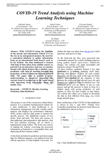
Data miningprocessKnowledgeDiscovery inDatabases: ProcessInterpretation/EvaluationEvaluate objectively on historical data,Data MiningKnowledgeKnowledgesubjectively with fraud analystsLearn decision trees, outputpredictions andPatternstree structurePreprocessingSelectionCreate class label,temporal featuresPreprocessedfirms DataExtract data about smallin aDatafew geographicTarget locationsUse public data fromNASD BrokerCheckDataadapted from:U. Fayyad, et al. (1995), “From Knowledge Discovery to DataMining: An Overview,” Advances in Knowledge Discovery andData Mining, U. Fayyad et al. (Eds.), AAAI/MIT PressCS590D13
Steps in the data mining process
Data mining process1. Application setup: Acquire relevant domainknowledge Assess user goals2. Data selection Choose data sources3. Data preprocessing Remove noise or outliers Handle missing values Account for time or otherchanges4. Data transformation Identify relevant attributes Find useful features Sample data Reduce dimensionality
Data mining process5. Data mining: Choose task (e.g.,classification, regression,clustering) Choose algorithms forlearning and inference Set parameters Apply algorithms to searchfor patterns of interest6. Interpretation/evaluation Assess accuracy of model/results Interpret model for end-users Consolidate knowledge7. Repeat.
Data selection
# download data from:# https://www.cs.purdue.edu/homes/neville/iris.dat# read in datad - read.table(file ‘iris.dat’,sep ',',header TRUE)summary(d)# histogramhist(d[,2], main 'Histogram of Sepal Width', xlab 'SepalWidth')# scatterplotplot(d[,c(1,3)],xlab 'Sepal Length',ylab 'Petal Length’)plot(d)
# feature constructionSepalArea - d[,1] * d[,2]PetalArea - d[,3] * d[,4]# add new features to data framed2 - cbind(d,SepalArea,PetalArea)# boxplotboxplot(d2 SepalLength d2 Class,d2,ylab 'Sepal Length’)boxplot(d2 SepalArea d2 Class,d2,ylab 'Sepal Area')# correlationcor(d2 SepalLength,d2 sepalArea)
Data transformation
Feature construction Create new attributes that can capture the important information in the datamore efficiently than the original attributes General methodologies: Attribute extraction (domain specific) Attribute transformations, i.e., mapping data to new space (e.g., PCA) Attribute combinations
Feature selection Select the most “relevant” subset of attributes May improve performance of algorithms due to overfitting Improves domain understanding Less resources to collect/use a smaller number of features Wrapper approach Features are selected as part of the mining algorithms Filter approach Features are selected before mining
Wrapper approach Consider all subsets of features, 2p if there are p features; features areselected according to a particular model score function (e.g., classificationaccuracy) Search over all subsets and find smallest set of features such that “best”model score does not significantly change For large p, exhaustive search is intractable so heuristic search is often used Examples: Forward, greedy selection — start with empty set and add features one ata time until no more improvement Backward, greedy removal — start with full set and remove features oneat a time until no further improvements Interleave forward and backward selection
Filter approach Select “useful” features before mining, using a score that measures a feature’sutility separate from model learning Find features on the basis of statistical properties such as association with theclass label Example: Calculate correlation of features with target class label, order all featuresby their score, choose features with top k scores Other scores: Chi-square, information gain, etc.
Dimensionality reduction Identify and describe the “dimensions” that underlie the data May be more fundamental than those directly measured but hidden to theuser Reduce dimensionality of modeling problem Benefit is simplification, it reduces the number of variables you have todeal with in modeling Can identify set of variables with similar behavior
Principal component analysis (PCA) High-level approach, given data matrix D with p dimensions: Preprocess D so that the mean of each attribute is 0, call this matrix X Compute pxp covariance matrix: X XT Compute eigenvectors/eigenvalues of covariance matrix:A A1 A : matrix of eigenvectors : diagonal matrix of eigenvaluesA are the principal component vectors (pxp matrix),a is a px1 column vector of projection weights Eigenvectorswhere each
Applying PCA New data vectors are formed by projecting the data onto the first few principalcomponents (i.e., top k eigenvectors)x [x1 , x2 , . . . , xp ] (original instance)A [a1 , a2 , . . . , ap ] (principal components)x01 a1 x pXa1j xjj 1···x0m am x pXj 1amj xj f or m pIf m p then data is transformedIf m p then transformation is lossyand dimensionality is reducedx0 [x01 , x02 , . . . , x0m ] (transformed instance)
Applying PCA (cont’) Goal: Find a new (smaller) set ofdimensions that captures most ofthe variability of the data Choose m p so projected datacaptures much of the varianceof original dataVariance Use scree plot to choose numberof dimensionsIndex
Example: EigenfacesPCA applied toimages of humanfaces.Reducedimensionality toset of basisimages.All other imagesare linear comboof these“eigenpictures”.Used for facialrecognition.First 40 PCA dimensions
PCA example on Iris data pcdat - princomp(d[,1:4]) summary(pcdat)Importance of components:Comp.1Comp.2Comp.3Comp.4Standard deviation2.0485788 0.49053911 0.27928554 0.153379074Proportion of Variance 0.9246162 0.05301557 0.01718514 0.005183085Cumulative Proportion 0.9246162 0.97763178 0.99481691 1.000000000 plot(pcdat)First component explains loadings(pcdat)92% of data variance40000100002000030000Choose m 10Comp.1 Comp.2 Comp.3 Comp.4SS loadings1.001.001.001.00Proportion Var0.250.250.250.25Cumulative Var0.250.500.751.00pcdatVariancesLoadings:Comp.1 Comp.2 Comp.3 Comp.4V1 0.362 -0.657 -0.581 0.317V2-0.730 0.596 -0.324V3 0.857 0.176-0.480V4 0.3590.549 0.751Comp.1Comp.2Comp.3Comp.4
···p using 1st component# Transform dataXpcdat loadings[,1]x0m am x amj xj f or m pV1V2V3V4j 10.36158968 -0.08226889 0.85657211 0.35884393x0 [x01 , x02 , . . . , x0m ] (transformed instance)pcaF - as.matrix(d[,1:4]) %*% pcdat loadings[,1]d3 - cbind(d2,pcaF)4.5 5.0 5.5 6.0 6.5 7.0 7.5 8.0Iris-setosaIris-virginicaTransformed data9j 18a1j xj7x01 a1 x pX6A [a1 , a2 , . . . , ap ] (principal components)5x [x1 , x2 , . . . , xp ] (original instance)4m 1, transform data to one dimensionOriginal data (1st variable)3PCA example on Iris data123
Machine learning
Descriptive vs. predictive modeling Descriptive models summarize the data Provide insights into the domain Focus on modeling joint distribution P(X) May be used for classification, but prediction is not the primary goal Predictive models predict the value of one variable of interest given knownvalues of other variables Focus on modeling the conditional distribution P( Y X ) or on modelingthe decision boundary for Y
Learning predictive models Choose a data representation Select a knowledge representation (a “model”) Defines a space of possible models M {M1, M2, ., Mk} Use search to identify “best” model(s) Search the space of models (i.e., with alternative structures and/orparameters) Evaluate possible models with scoring function to determine the modelwhich best fits the data
Knowledge representation Underlying structure of the model or patterns that we seek from the data Defines space of possible models for algorithm to search over Model: high-level global description of dataset “All models are wrong, some models are useful”G. Box and N. Draper (1987) Choice of model family determines space of parameters and structure Estimate model parameters and possibly model structure from training data
Classification treeBrokerAge 27Current CoWorkerCount 8Current BranchMode(Location) NY703564Current FirmAvg(Size) 12DisclosureCount(Yr 1995) 0Past CoWorkerCount(Gender M) 1510DisclosureCount 5Current BranchMode(Location) AZ7Model space:all possible decision trees1792189DisclosureCount(Type CC) 0Past FirmAvg(Size) 90200Past FirmMax(Size) 100049Past CoWorkerCount 35Current RegulatorMode(Status) RegBrokerYears In Industry 16334249554
Scoring functions Given a model M and dataset D, we would like to “score” model M withrespect to D Goal is to rank the models in terms of their utility (for capturing D)and choose the “best” model Score function can be used to search over parameters and/ormodel structure Score functions can be different for: Models vs. patterns Predictive vs. descriptive functions Models with varying complexity (i.e., number parameters)
Predictive scoring functions Assess the quality of predictions for a set of instances Measures difference between the prediction M makes for aninstance i and the true class label value of iS(M ) NtestXi 1Sum overexamples d f (x(i); M ), y(i)Distance betweenpredicted and truePredictedclass labelfor item i Trueclass labelfor item i
What space are we searching?Learned model ( 0 0.8, 1 0.4)XModelScoreModel spaceAlex Holehuse, Notes from Andrew Ng’s Machine Learning Class, http://www.holehouse.org/mlclass/01 02 Introduction regression analysis and gr.html
Searching over models/patterns Consider a space of possible models M {M1, M2, ., Mk} with parameters θ Search could be over model structures or parameters, e.g.: Parameters: In a linear regression model, find the regressioncoefficients (β) that minimize squared loss on the training data Model structure: In a decision trees, find the tree structure thatmaximizes accuracy on the training data
Decision trees
Tree models Easy to understand knowledgerepresentation Can handle mixed variables Recursive, divide and conquerlearning method Efficient inference
Tree learning Top-down recursive divide and conquer algorithm Start with all examples at root Select best attribute/feature Partition examples by selected attribute Recurse and repeat Other issues: How to construct features When to stop growing Pruning irrelevant parts of the tree
FraudAgeDegreeStartYrSeries7 22Y2005N-25N2003Y-31Y1995Y-27Y1999Y 24N2006N-29N2003NYchoose split on Series7Score each attribute splitfor these instances:Age, Degree, StartYr, StartYrSeries7-25N2003Y 22Y2005N-31Y1995Y 24N2006N-27Y1999Y-29N2003NYchoose split on Age 28ScoreN each attribute splitfor these instances:Age, Degree, tartYrSeries7-29N2003N 22Y2005N 24N2006N
Tree models Most well-known systems CART: Breiman, Friedman, Olshen and Stone ID3, C4.5: Quinlan How do they differ? Split scoring function Stopping criterion Pruning mechanism Predictions in leaf nodes
Scoring functions: Local split value
Choosing an attribute/feature Idea: a good feature splits the examples into subsets that distinguish amongthe class labels as much as possible. ideally into pure sets of "all positive" or"all negative"
predictionBayesian ClassificationInstance Based MethodsClassification by decision tree inductionClassification by Neural NetworksClassification by Support Vector MachinesCS590D30(SVM) How much doesa feature split decrease the entropy?PredictionInformation gain Training Datasetage 30 3031 40 40 40 4031 40 30 30 40 3031 4031 40 40income student credit airlowyes fairlowyes excellentlowyes excellentmediumnofairlowyes fairmediumyes fairmediumyes excellentmediumnoexcellenthighyes fairmediumnoexcellentCS590Dbuys py(D) -9/14 log 9/14 -5/14 log 5/14 0.94003167
Information gainEntropy(Income high) -2/4 log 2/4 -2/4 log 2/4 1IncomeHighnonoyesyesMed LowyesnoyesyesyesnoyesnoyesyesEntropy(Income med) -4/6 log 4/6 -2/6 log 2/6 0.9183Entropy(Income low) -3/4 log 3/4 -1/4 log 1/4 0.8113Gain(D,Income) 0.9400 - (4/14 [1] 6/14 [0.9183] 4/14 [0.8113]) 0.02968
Tree learning Top-down recursive divide and conquer algorithm Start with all examples at root Select best attribute/feature Partition examples by selected attribute Recurse and repeat Other issues: How to construct features When to stop growing Pruning irrelevant parts of the tree
When to stop growing Full growth methods All samples for at a node belong to the same class There are no attributes left for further splits There are no samples left What impact does this have on the quality of the learned trees? Trees overfit the data and accuracy decreases Pruning is used to avoid overfitting
Pruning Postpruning Use a separate set of examples to evaluate the utility of pruning nodesfrom the tree (after tree is fully grown) Prepruning Apply a statistical test to decide whether to expand a node Use an explicit measure of complexity to penalize large trees (e.g.,Minimum Description Length)
Algorithm comparison CART C4.5 Evaluation criterion:Gini index Evaluation criterion:Information gain Search algorithm:Simple to complex,hill-climbing search Search algorithm:Simple to complex,hill-climbing search Stopping criterion:When leaves are pure Stopping criterion:When leaves are pure Pruning mechanism:Cross-validation to selectgini threshold Pruning mechanism:Reduce error pruning
Learning CART decision trees in R
# install ")library(rpart.plot)# learn CART tree with default parametersdTree - rpart(Class SepalLength SepalWidth PetalLength PetalWidth SepalArea PetalArea pcaF, method “class", data d3)summary(dTree)# display learned treeprp(dTree)prp(dTree,type 4, extra 1)# explore settingsdTree2 - rpart(Class SepalLength SepalWidth PetalLength PetalWidth SepalArea PetalArea pcaF, method “class", data d3,parms list(split "information"))dTree3 - rpart(Class SepalLength SepalWidth PetalLength PetalWidth SepalArea PetalArea pcaF, method "class", data d3,control rpart.control(minsplit 5))
Evaluation
Empirical evaluation Given observed accuracy of a model on limited data, how well does thisestimate generalize for additional examples? Given that one model outperforms another on some sample of data, how likelyis it that this model is more accurate in general? When data are limited, what is the best way to use the data to both learn andevaluate a model?
Evaluating classifiers Goal: Estimate true future error rate When data are limited, what is the best way to use the data to both learn andevaluate a model? Approach 1 Reclassify training data to estimate error rate
Approach 1YX1X2F(X)YX1X2Score: 83%ModelDataSetDataSetTypically produces a biased estimate of future error rate -- why?
Learning curves Goal: See how performance improves with additional training data From dataset set S, where S n For i [10, 20, . ,100] Randomly sample i% of S to construct sample S’ Learn model on S’ Evaluate model Plot training set size vs. accuracy
Size of dataset
How does performance change whenmeasured on disjoint test set?
Size of dataset
Approach 2YYX1X1X2X2ModelTraining setYX1 X2F(X)YX1 X2Score: 77%DataSetTest setTest setEstimate will vary due to size and makeup of test set
Evaluating classifiers (cont) Approach 2:0.60.8Algorithm AAlgorithm B0.00.20.4Error Problem: this is a pointestimate of the error onone subset1.0 Partition D0 into twodisjoint subsets, learnmodel on one subset,measure error on the othersubset0200400Training Set Size600800
Overlapping test sets are dependent Repeated sampling of test sets leads to overlap (i.e., dependence) among testsets. this will results in underestimation of variance Standard errors will be biased ifperformance is estimated fromoverlapping test sets (Dietterich’98) Recommendation:Use cross-validation to eliminatedependence between test setsA A
Evaluating classification algorithms A and B Use k-fold cross-validation to get k estimates of error for MA and AccA.6AccB.6 Set of errors estimated over the test set folds provides empirical estimate ofsampling distribution Mean is estimate of expected error
# package with helper methodsinstall.packages("caret")library(caret)# partition data into 80% training and 20% test settrainIndex - createDataPartition(d3 SepalLength, times 1, p 0.8, list FALSE)dTrain - d3[ trainIndex,]dTest - d3[-trainIndex,]# learn model from training, evaluate on testdtTrain - rpart(Class SepalLength SepalWidth PetalLength PetalWidth SepalArea PetalArea pcaF, method "class", data dTrain,control rpart.control(minsplit 5))testPreds - predict(dtTrain, dTest, type "class")# evaluateconfusionMatrix(testPreds, dTest Class)
# calculate learning curveallResultsTr - matrix(numeric(0), 0,2)allResultsTe - matrix(numeric(0), 0,2)trainSetSizes - c(0.025,0.05,0.1,0.2,0.4,0.8)for(i in trainSetSizes){trainIndex - createDataPartition(d3 SepalLength,times 1,p i,list FALSE)dTrain - d3[ trainIndex,]dTest - d3[-trainIndex,]dTree - rpart(Class SepalLength SepalWidth PetalLength PetalWidth SepalArea PetalArea pcaF, method "class", data dTrain,control rpart.control(minsplit 5))# evaluate on test settestPreds - predict(dTree, dTest, type "class")evalResults - confusionMatrix(testPreds, dTest Class)tmpAcc - evalResults overall[1]allResultsTe - rbind(allResultsTe, as.vector(c(i,tmpAcc)))# evaluate on training settrainPreds - predict(dTree, dTrain, type "class")evalResults2 - confusionMatrix(trainPreds, dTrain Class)tmpAcc2 - evalResults2 overall[1]allResultsTr - rbind(allResultsTr, as.vector(c(i,tmpAcc2)))}
Ensemble methods
Ensemble methods Motivation Too difficult to construct a single model that optimizes performance (why?) Approach Construct many models on different versions of the training set andcombine them during prediction Goal: reduce bias and/or variance
Conventional classificationX: attributesY: class label
Ensemble classification92
Relative Performance Examples: 5 Algorithms on 6 DatasetsError Relative to Peer Techniques (lower is better)1.00.90.80(with Stephen Lee, U. Idaho, 1997)Neural NetworkLogistic RegressionLinear Vector QuantizationProjection Pursuit RegressionDecision Tree.70.60.50.40.30.20.10.00DiabetesGaussian 2004 Elder Research, rce: Top Ten Data Mining Mistakes, John Edler, Edler Research)
Essentially every Bundlingensemble method improves performanceError Relative to Peer Techniques (lower is better)1.00.90.80.70.60.50.40Advisor PerceptronAP weighted averageVoteAverage.30.20.10.00DiabetesGaussian 2004 Elder Research, rce: Top Ten Data Mining Mistakes, John Edler, Edler Research)
Ensemble design
Ensemble designTREATMENT OF INPUT DATA sampling variable selection
Ensemble designTREATMENT OF INPUT DATACHOICE OF BASE CLASSIFIER sampling decision tree variable selection perceptron
Ensemble designTREATMENT OF INPUT DATACHOICE OF BASE CLASSIFIERPREDICTION AGGREGATION sampling decision tree averaging variable selection perceptron weighted vote
Bagging Bootstrap aggregating Main assumption Combining many unstable predictors in an ensemble produces a stablepredictor (i.e., reduces variance) Unstable predictor: small changes in training data produces large changesin the model (e.g., trees) Model space: non-parametric, can model any function if an appropriate basemodel is used
BaggingTREATMENT OF INPUT DATACHOICE OF BASE CLASSIFIERPREDICTION AGGREGATION sample with replacement unstable predictore.g., decision tree averaging
Bagging Given a training data set D {(x1,y1),., (xN,yN)} For m 1:M Obtain a bootstrap sample Dm by drawing N instanceswith replacement from DSample to createaltered training data Learn model Mm from Dm To classify test instance t, apply each model Mm to t and use majoritypredication or average prediction Models have uncorrelated errors due to difference in training sets(each bootstrap sample has 68% of D)
Random forests Given a training data set D {(x1,y1),., (xN,yN)} For m 1:M Obtain a bootstrap sample Dm by drawing N instanceswith replacement from D Learn decision tree Mm from Dmusing k randomly selected features at each split To classify test instance t, apply each model Mm to t and use majoritypredication or average prediction
st)# random forest ensembledForest - randomForest(Class SepalLength SepalWidth PetalLength PetalWidth SepalArea PetalArea pcaF,method “class", data d3)# view resultsprint(dForest)# importance of each predictorimportance(dForest)
# calculate learning curve for random forestallResultsTe - matrix(numeric(0), 0,2)trainSetSizes - c(0.025,0.05,0.1,0.2,0.4,0.8)for(i in trainSetSizes){trainIndex - createDataPartition(d3 SepalLength, times 1, p i, list FALSE)dTrain - d3[ trainIndex,]dTest - d3[-trainIndex,]dForest - randomForest(Class SepalLength SepalWidth PetalLength PetalWidth SepalArea PetalArea pcaF,method "class",data d3)# evaluate on test settestPreds - predict(dForest, dTest, type "class")evalResults - confusionMatrix(testPreds, dTest Class)tmpAcc - evalResults overall[1]allResultsTe - rbind(allResultsTe, as.vector(c(i,tmpAcc
Data mining process 6 CS590D 12 Data Mining: Classification Schemes General functionality – Descriptive data mining – Predictive data mining Different views, different classifications – Kinds of data to be mined – Kinds of knowledge to be discovered – Kinds of techniqu