Transcription
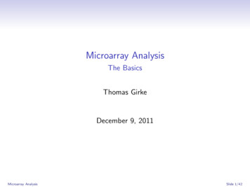
Microarray AnalysisThe BasicsThomas GirkeDecember 9, 2011Microarray AnalysisSlide 1/42
TechnologyChallengesData AnalysisData DepositoriesR and BioConductorHomework AssignmentMicroarray AnalysisSlide 2/42
OutlineTechnologyChallengesData AnalysisData DepositoriesR and BioConductorHomework AssignmentMicroarray AnalysisTechnologySlide 3/42
Microarray and Chip TechnologyDefinitionHybridization-based technique that allows simultaneousanalysis of thousands of samples on a solid substrate.ApplicationsTranscriptional ProfilingGene copy numberResequencingGenotypingSingle-nucleotide polymorphismDNA-protein interaction (e.g.: ChIP-on-chip)Gene discovery (e.g.: Tiling arrays)Identification of new cell linesEtc.Related technologiesProtein arraysCompound arraysMicroarray AnalysisTechnologySlide 4/42
Why Microarrays?Simultaneous analysis of thousands of genesDiscovery of gene functionsGenome-wide network analysisAnalysis of mutants and transgenicsIdentification of drug targetsCausal understanding of diseasesClinical studies and field trialsMicroarray AnalysisTechnologySlide 5/42
Different Types of MicroarraysSingle channel approachesAffymetrix gene chipsMacroarraysMultiple channel approachesDual color (cDNA) microarraysSpecialty approachesBead arrays: Lynx, Illumina, .PCR-based profiling: CuraGen, .Microarray AnalysisTechnologySlide 6/42
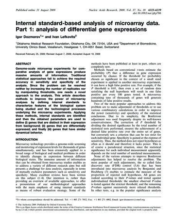
Dual Color MicroarraysMicroarray AnalysisTechnologySlide 7/42
Affymetrix DNA ChipsMicroarray AnalysisTechnologySlide 8/42
OutlineTechnologyChallengesData AnalysisData DepositoriesR and BioConductorHomework AssignmentMicroarray AnalysisChallengesSlide 9/42
Profiling Chips Monitor Differences of mRNA LevelsEfficient strategy for down-stream follow-up experimentsimportant!Microarray AnalysisChallengesSlide 10/42
Strategies to Validate Array HitsReal-time PCR, Northern, etc.Transgenic testsKnockout plants and/or activation tagged linesProtein profilingMetabolic profilingOther tests: in situ hybs, biochemical and physiological testsIntegration with sequence, proteomics and metabolicdatabasesMicroarray AnalysisChallengesSlide 11/42
Sources of Variation in Transcriptional ProfilingExperimentsEvery step in transcriptional profiling experiments cancontribute to the inherent ’noise’ of array data.Variations in biosamples, RNA quality and target labeling arenormally the biggest noise introducing steps in arrayexperiments.Careful experimental design and initial calibration experimentscan minimize those challenges.Microarray AnalysisChallengesSlide 12/42
Experimental DesignBiological questions:Which genes are expressed in a sample?Which genes are differentially expressed (DE) in a treatment, mutant,etc.?Which genes are co-regulated in a series of treatments?Selection of best biological samples and referenceComparisons with minimum number of variablesSample selection: maximum number of expressed genesAlternative reference: pooled RNA of all time points (saves chips)Develop validation and follow-up strategy for expected expression hitse.g. real-time PCR and analysis of transgenics or mutantsChoose type of experimentcommon reference, e.g.: S1 x S1 T1, S1 x S1 T2paired references, e.g.: S1 x S1 T1, S2 x S2 T1loop & pooling designsmany other designsAt least three (two) biological replicates are essentialBiological replicates: utilize independently collected biosamplesTechnical replicates: utilize often the same biosample or RNA poolMicroarray AnalysisChallengesSlide 13/42
OutlineTechnologyChallengesData AnalysisData DepositoriesR and BioConductorHomework AssignmentMicroarray AnalysisData AnalysisSlide 14/42
Basic Data Analysis StepsImage Processing: transform feature and background pixelinto intensity valuesTransformationsRemoval of flagged values (optional)Detection limit (optional)Background subtractionTaking logarithmsNormalizationIdentify EGs and DEGsWhich genes are expressed?Which genes are differentially expressed?Cluster analysis (time series)Which genes have similar expression profiles?Promoter analysisIntegration with functional information: pathways, etc.Microarray AnalysisData AnalysisSlide 15/42
Image AnalysisOverall slide qualityGrid alignment (linkage between spots and feature IDs)Signal quantification: mean, median, threshold, etc.Local backgroundManual spot flaggingExport to text fileImage analysis software (selection)ScanAlyze (http://rana.lbl.gov/EisenSoftware.htm)TIGR SpotFinder (http://www.tigr.org/software/)Microarray AnalysisData AnalysisSlide 16/42
Background CorrectionFiltering (optional)Intensities below detection limitNegative intensitiesSpacial quality issuesBackground correctionBG consists of non-specific hybridization and backgroundfluorescenceIf BG is higher than signal: (1) remove values, (2) set signal tolowest measured intensity, (3) many other approachesBG subtractionLocal backgroundGlobal backgroundNo background subtractionBackground subtraction can cause ratio inflation, thereforebackground corrected intensities below threshold are often setto threshold or similar value.Microarray AnalysisData AnalysisSlide 17/42
NormalizationNormalization is the process of balancing the intensities of thechannels to account for variations in labeling and hybridizationefficiencies. To achieve this, various adjustment strategies are usedto force the distribution of all ratios to have a median (mean) of 1or the log-ratios to have a median (mean) of 0.Microarray AnalysisData AnalysisSlide 18/42
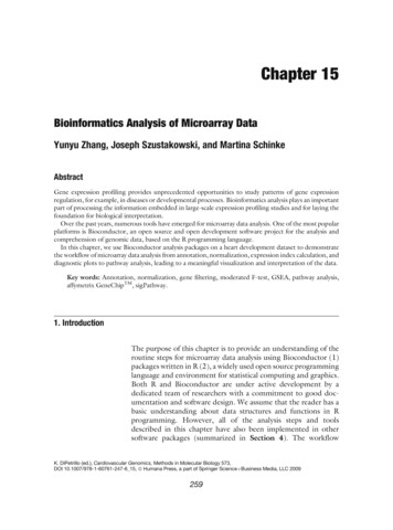
Log Transformation: Scatter PlotsReasons for working with log-transformed intensities and ratios(1) spreads features more evenly across intensity range(2) makes variability more constant across intensity range(3) results in close to normal distribution of intensities and experimental errorsMicroarray AnalysisData AnalysisSlide 19/42
Log Transformation: HistogramsDistribution of log transformed data is closer to being bell-shapedMicroarray AnalysisData AnalysisSlide 20/42
Normalization If Large Fraction of Genes IS DEMinimize normalization requirements (dynamic range limits)Pre-scanning: hybridize equal amounts of labelDuring scanning: balance average intensities through laserpower and PMP adjustmentsNormalization if large fraction of genes is DESpike-in controlsHousekeeping controlsDetermine constant feature setMicroarray AnalysisData AnalysisSlide 21/42
Normalization If Large Fraction of Genes IS NOT DEGlobal Within-Array NormalizationMultiply one channels with normalization factor Ch2 x mCh1/mCh2 (treats both channels differently)Linear regression fit of log2(Ch2) against log2(Ch1) adjust Ch1 with fitted values (treats both channelsdifferently)Linear regression fit of log2(ratios) against avg log2(int) subtract fitted value from raw log ratios (treats bothchannels equally)Non-linear regression fit of log2(ratios) against avg log2(int)Most commonly used: Loess (locally weighted polynomial)regression joins local regressions with overlapping windows tosmooth curve subtract fitted value on Loess regression from raw logratios (treats both channels equally)Microarray AnalysisData AnalysisSlide 22/42
MA PlotsMicroarray AnalysisData AnalysisSlide 23/42
Normalization If Large Fraction of Genes IS NOT DESpacial Within-Array NormalizationAll of the above methods can be used to correct for spacialbias on the array. Examples:Block or Print Tip Loess2D Loess RegressionMicroarray AnalysisData AnalysisSlide 24/42
Normalization If Large Fraction of Genes IS NOT DEBetween-Array NormalizationTo compare ratios between dual-color arrays or intensitiesbetween single-color arraysScaling log(rat) - mean log(rat) or log(int) - mean log(int) Result: mean 0Centering (z-value) [rat - mean(rat)] / [STD] or [int - mean(int)] / [STD] Result: mean 0, STD 1Distribution Normalization (apply to group of arrays!) (1) Generate centered data, (2) sort each array byintensities, (3) calculate mean for sorted values across arrays,(4) replace sorted array intensities by corresponding meanvalues, (5) sort data back to original order Result: mean 0, STD 1, identical distribution betweenarraysMicroarray AnalysisData AnalysisSlide 25/42
Box Plots for Between-Array Normalization StepsMicroarray AnalysisData AnalysisSlide 26/42
Analysis Methods for Affymetrix Gene ChipsMethodMAS5BG AdjustregionaladjustmentNormalizationscaling byconstantMM Correctsubtractidealized MMProbeset SummaryTukey biweightaveragegcRMAby GCcontentquantilenormalization/robust fit oflinear t fit oflinear modelVSN/variancestabilizing TF/robust fit oflinear modeldChip/by invariantset/multiplicativemodeldChip.mm/by invariantsetsubtractmismatchmultiplicativemodelQin et al. (2006), BMC Bioinfo, 7:23.ReverencesMAS 5.0: Affymetrix Documentation: MAS5PLIER: Affymetrix Documentation: PLIER, not included heregcRMA: Wu et al. (2004), JASA, 99, 909-917.RMA: Irizarry et al. (2003), Nuc Acids Res, 31, e15.VSN: Huber et al. (2002), Bioinformatics, 18, Suppl I S96-104.dChip & dChip.mm: Li & Wong (2001), PNAS, 98, 31-36.Microarray AnalysisData AnalysisSlide 27/42
Performance Comparison of Affy MethodsQin et al. (2006), BMC Bioinfo, 7:23: 24 RNA samples hybridized to chips and 47genes tested by qRT-PCR, plot shows PCC for 6 summary contrasts of 6 methods.MAS5, gcRMA, and dChip (PM-MM) outperform the other methods. PLIER notincluded here.Microarray AnalysisData AnalysisSlide 28/42
Analysis of Differentially Expressed GenesAdvantages of statistical test over fold change threshold forselecting DE genesIncorporates variation between measurementsEstimate for error rateDetection of minor changesRanking of DE genesApproachesParametric test: t-testNon-parametric tests: Wilcoxon sign-rank/rank-sum testsBootstrap analysis (boot package)Significance Analysis of Microarrays (SAM)Linear Models of Microarrays (LIMMA)Rank ProductANOVA and MANOVA (R/maanova)Multiplicity of testing: p-value adjustmentsMethods: fdr, bonferroni, etc.Microarray AnalysisData AnalysisSlide 29/42
OutlineTechnologyChallengesData AnalysisData DepositoriesR and BioConductorHomework AssignmentMicroarray AnalysisData DepositoriesSlide 30/42
Microarray Databases and DepositoriesNCBI GEO: http://www.ncbi.nlm.nih.gov/geoMicroarray @ EBI: http://www.ebi.ac.uk/microarraySMD: http://genome-www5.stanford.eduMany OthersMicroarray AnalysisData DepositoriesSlide 31/42
OutlineTechnologyChallengesData AnalysisData DepositoriesR and BioConductorHomework AssignmentMicroarray AnalysisR and BioConductorSlide 32/42
Why Using R and BioConductor for Array Analysis?Complete statistical package and programming languageUseful for all bioscience areasPowerful graphicsAccess to fast growing number of analysis packagesIs standard for data mining and biostatistical analysisTechnical advantages: free, open-source, available for all OSsBooks & DocumentationsimpleR - Using R for Introductory Statistics (Gentleman etal., 2005)Bioinformatics and Computational Biology Solutions Using Rand Bioconductor (John Verzani, 2004)UCR Manual (Thomas Girke)Microarray AnalysisR and BioConductorSlide 33/42
Installation1Install R binary for your operating system from:http://cran.at.r-project.org2Install the required packages from BioConductor by executingthe following commands in R: source("http://www.bioconductor.org/biocLite.R") biocLite() biocLite(c("GOstats", "Ruuid", "graph", "GO", "Category","plier", "affylmGUI", "limmaGUI", "simpleaffy","ath1121501", "ath1121501cdf", "ath1121501probe", "biomaRt","affycoretools"))Microarray AnalysisR and BioConductorSlide 34/42
R Essentials# General R command syntax object - function(arguments)# Execute an R script source("homework script.R")# Finding help ?function# Load a library library(affy)# Summary of all functions within a library library(help affy)# Load library manual (PDF file) openVignette()Microarray AnalysisR and BioConductorSlide 35/42
OutlineTechnologyChallengesData AnalysisData DepositoriesR and BioConductorHomework AssignmentMicroarray AnalysisHomework AssignmentSlide 36/42
Obtain Sample Data from GEORetieve the ”Arabidopsis light treatment series” (GSE5617)from GEO with the following query:Arabidopsis[Organism] AND Atgenexpress[Title] ANDlight[Title]Download the following Cel files from this GSE5617 M131195.CELGSM131211.CELBatch download:GEO CEL.zipMicroarray AnalysisHomework AssignmentSlide 37/42
Define Replicates and TreatmentsGenerate targets.txt file and save it in your working directory.It should contain the following content:NameDS REP1DS REP2DS REP3PS REP1PS REP2PS REP3BS REP1BS REP2BS REP3Microarray 181.CELGSM131195.CELGSM131211.CELHomework AssignmentTargetdark45mdark45mdark45mred1m dark44mred1m dark44mred1m dark44mblue45mblue45mblue45mSlide 38/42
Homework TasksA. Generate expression data with RMA, GCRMA and MAS 5.0.Create box plots for the raw data and the RMA normalizeddata.B. Perform the DEG analysis with the limma package anddetermine the differentially expressed genes for eachnormalization data set using as cutoff an adjusted p-value of 0.05. Record the number of DEGs for each of the threenormalization methods in a summary table.C. Create for the DEG sets of the three sample comparisons avenn diagram (adjusted p-value cutoff 0.05).D. Generate a list of genes (probe sets) that appear in all threefiltered DEG sets (from B.). Command summary: source(”homework script.R”)Microarray AnalysisHomework AssignmentSlide 39/42
R Commands for Normalization# Load required libraries library(affy); library(limma); library(gcrma)# Open limma manual limmaUsersGuide()# Import experiment design information from targets.txt targets - readTargets("targets.txt")# Import expression raw data and store them in AffyBatch object data - ReadAffy(filenames targets FileName)# Normalize the data with the RMA method and store results in exprSetobject eset - rma(data) # RMA and GCRMA store log2 intensities and MAS5absolute intensities.# Print the analyzed file names pData(eset)# Export all affy expression values to a tab delimited text file write.exprs(eset, file "affy all.xls")Microarray AnalysisHomework AssignmentSlide 40/42
R Commands for Differential Expression Analysis# Create appropriate design matrix and assign column names design - model.matrix( -1 factor(c(1,1,1,2,2,2,3,3,3)));colnames(design) - c("S1", "S2", "S3")# Create appropriate contrast matrix for pairwise comparisons contrast.matrix - makeContrasts(S2-S1, S3-S2, S3-S1, levels design)# Fit a linear model for each gene based on the given series of arrays fit - lmFit(eset, design)# Compute estimated coefficients and standard errors for a given set ofcontrasts fit2 - contrasts.fit(fit, contrast.matrix)# Compute moderated t-statistics and log-odds of differential expressionby empirical Bayes shrinkage of the standard errors towards a commonvalue fit2 - eBayes(fit2)# Generate list of top 10 DEGs for first comparison topTable(fit2, coef 1, adjust "fdr", sort.by "B", number 10)Microarray AnalysisHomework AssignmentSlide 41/42
Online ManualContinue on online manual.Microarray AnalysisHomework AssignmentSlide 42/42
simpleR - Using R for Introductory Statistics(Gentleman et al., 2005) Bioinformatics and Computational Biology Solutions Using R and Bioconductor(John Verzani, 2004) UCR Manual(Thomas Girke) Microarray