Transcription
Management AccountingInventory Decision-MakingTo be successful, most businesses other than service businesses are requiredto carry inventory. In these businesses, good management of inventory is essential.The management of inventory requires a number of decisions. Poor decision makingregarding inventory can cause:1. Loss of sales because of stock outs.2. Depending on circumstances, inadequate production for a period of time.3. Increases in operating expenses due to unnecessary carrying costs orloss from discarding obsolete inventory.4. An increase in the per unit cost of finished goods.Of all the activities in a manufacturing business, inventory creation is the mostdynamic and certainly the most visible activity. In one sense, inventory involves allproduction activity from the purchase of raw materials to the delivery of finished goodsinventory to the customer. The financial accounting for inventory is concerned primarilywith determining the correct count and the assignment of historical cost. However,from a management accounting viewpoint, the central focus is on manufacturing theright amounts at the lowest cost consistent with a quality product. From a financialviewpoint, poor management of inventory can adversely affect cash flow. Also,excessive inventory can cause a decrease in ROI. An over stock of inventory causestotal assets to be larger and certain expenses to increase. Consequently, in additionto a reduced cash flow, the effect of poor inventory management can be a lower rateof return. 195
196 CHAPTER ELEVEN Inventory Decision-MakingFinished goods inventory represents the company’s product for available for saleat a given point in time. A certain amount of inventory must be available at all times inorder to have an effective marketing operation. The poor management of inventory,including finished goods, is often reflected in the use of terms such as such as stockouts, back orders, decrease in inventory turnover, lost sales, and inadequate safetystock.The existence of inventory results in expenses other than the cost of inventoryitself which typically are categorized as:1. Carrying costs2. Purchasing costs.Inventory is a term that may mean finished goods, materials, and work in process.In a manufacturing business, there is a logical connection between these three typesof inventory:MaterialsLaborOverheadÆ Work in ProcessÆ Finished goodsÆ Cost of goods soldTo have finished goods inventory, production must take place at a rate greaterthan sales. Inventory decisions have a direct impact on production. For example, adecision to increase safety stock means that the production rate must increase untilthe desired level of safety stock is achieved.From an accounting standpoint, there are two main areas of concern. First, froma financial accounting viewpoint, the main accounting problems concern:1.2.3.4.The flow of costs (FIFO, LIFO, average cost)Use of a type of inventory costing method (periodic or perpetual)Taking of physical inventories.Techniques for estimating inventoryFrom a financial accounting viewpoint, the cost assigned to inventory directlyaffects net income. If ending inventory is overstated, then net income is overstatedand conversely, if ending inventory is understated then net income is understated.Also, the use of direct costing rather than absorption costing can affect net incomeas discussed in chapter 6. From a management accounting viewpoint, there arevariety of inventory decisions that affect net income. Decisions regarding inventorycan be placed in two general categories: (1) those decisions that affect the quantityof inventory and (2) those decisions that affect the per unit cost of inventory.Decisions that affect the quantity of inventory1. Order size2. Number of orders3. Safety stock4. Lead time5. Planned production
Management AccountingDecisions that affect the cost per unit of inventory1. Suppliers of raw material (list price and discounts)2. Order size (quantity discounts)3. FreightIn addition, decisions pertaining to labor and overhead also indirectly affect the perunit cost of inventory. In a manufacturing business, the costs of labor and overheaddo not become operating expenses until the manufacturing costs appear as partof cost of goods sold. Labor and overhead costs are deferred in inventory until theinventory has been sold.In this chapter, the main focus of discussion will be the following inventorydecisions:1. Production budget2. Order size for raw materials3. Number of times to order for raw materials4. Reorder point5. Safety stockProduction Budget DecisionThe production budget was discussed in some detail in chapter 8. The productionbudget decision is of utmost importance. If the production budget is inadequate, thenstock outs will occur. If the production budget is too large, then unnecessary carryingcosts will be incurred. The production budget format as presented previously was:Production BudgetFor the Quarter Ending March 31, 20xxSales forecastBack ordersDesired ending Finished Goods InventoryFinished goods (BI) 100,0005,00020,00025,00010,000 115,000The key to a good production management is an accurate sales forecast. Withouta reliable sales forecast, the production process is likely to be chaotic and have asignificant negative impact on sales. A good production budget is one that meets thecurrent sales demand plus provides for an adequate planned safety stock. Also, inthe preparation of the purchases budget, decisions for the desired levels of safetystock in materials must be made. The production budget determines the need forplant capacity. If the current production budget exceeds existing plant capacity, thenways to increase plant capacity must be considered. Increasing plant capacity mayinvolve scheduling overtime or a second shift or even purchasing and installing moreproduction equipment and hiring additional labor. 197
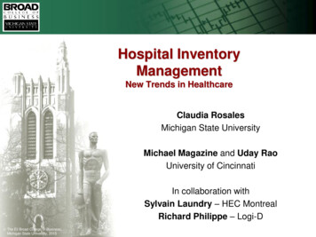
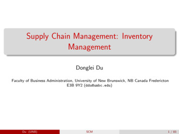
198 CHAPTER ELEVEN Inventory Decision-MakingPurchase of Materials DecisionThe main management accounting tool that may be used to make inventorypurchase decisions is the EOQ model. This tool recognizes that there are two majordecisions regarding the materials inventory: (1) orders size and (2) number of orders.There are consequently two major questions:1. How many units should be purchased each time a purchase is made(order size)?2. How many purchases should be made (number of orders)?To understand an EOQ model, it is essential that the concept of average inventorybe understood. Inventory is never static and is constantly rising and falling over time,even in the very short term. Inventory, for example, rises when raw materials arepurchased and falls when raw material is used. Because inventory in a business isconstantly changing, it is necessary to think in terms of average inventory levels.The high points and low points of inventory are easy to explain and illustrate, ifa purchasing policy is consistently applied and the rate of usage of raw materialis uniform. Inventory is at its highest and lowest levels when a new shipment ofmaterial arrives. Theoretically, in absence of a need for safety stock, a new shipmentshould arrive at the moment inventory reaches zero. Immediately, upon arrival of anew shipment, inventory is then at its highest level again. To illustrate, assume thateach purchase order placed is for 18,000 units at 5.00 per unit and that usage ofraw materials is uniform at 300 units of material per day. If production and usageof material takes place every day, then a shipment of material should last 60 days.These conditions may be illustrated as follows:Figure 11-1 Graphical Illustration of Average 240300360Work DaysIn terms of dollars, the amount invested in inventory would fluctuate between 90,000 and zero. In this example, the average inventory would be 9,000 computedas follows:Order sizeAverage Inventory –––––––––(1)2
Management AccountingAt its highest level inventory would be 18,000 units and at its lowest level inventorywould be 0. Based on the above equation average inventory is:AI (18,000 0)/ 2 9,000The major factor here that affects the level of inventory is order size ( the numberof units purchased in each order). If demand for materials for a full year is 108,000units, then the extremes for purchasing could be one large order of 108,000 or108,000 orders of one unit per order. Given these extremes, then average inventorycould be as low as .5 unit (1 /2) or as large as 54,000 (108,000 / 2). The best ordersize, as will be explained and illustrated now, is determined by the cost of ordering(purchasing) and the cost of carrying inventory.Purchasing CostThe purchase of materials or parts necessary to make a finished productinvolves a process that needs to be understood. The process begins with a purchaserequisition and finally ends with payment of the materials purchases. This processmay be illustrated as ofÆOrderReceiving andPreparationInspection ofof VoucherÆÆorderPayment ofPurchaseÆandAccountingThe cost of placing an order, therefore, consists of the following:1. Cost of preparing purchase requisition2. Cost of preparing purchase order3. Delivery of order (postage, telephone time, filing)4. Receiving of purchased materials (inspection, storing, receivingreport.5. Accounting costs (preparing vouchers and recording time)It is important to remember that the cost of the inventory itself is not a purchasingcost. The purchase of inventory is typically recorded to the materials purchasesaccount and is treated as a separate and distinct cost.The number of times an order is placed is to some extent discretionary. To illustrate,assume that the K. L. Widget Company has determined that for the current quarter100,000 units of raw material Y need to be purchased. Two extreme possibilitiespresent themselves. The first one is to simply buy one unit at a time and purchase100,000 times. The second extreme is to make 1 large order of 100,000 units.Between purchasing one unit at a time or buying one unit at a time 100,000 times,there is a large number of possibilities between an order size of 1 and 100,000.It is obvious that each time an order is placed some purchasing costs are incurred,and that as the number of orders placed increases, the total cost of purchasingincreases. To use a simple example, if you enjoy eating a sandwich at lunch each 199
200 CHAPTER ELEVEN Inventory Decision-Makingday and you make your own sandwiches, then you must purchase bread and say apackage of sliced ham. Then, at a minimum, you must purchase one loaf of breadand a package of sliced ham which, for example purposes here, can last for oneweek. You must then visit your grocery store once a week. This means that for afull year you would make a minimum of 52 trips a year. However, the other extremealternative would be to purchase a full year’s worth of bread and ham and, therefore,make only one trip per year. If the grocery store was 5 miles away and at a costof 50 per mile, each trip will cost you 5.00 per trip or 260 per year. However,purchasing one time per year, then means you have a carrying or storage problem.You would have to have space to store 52 loaves of bread and packages of slicedhim. Assuming you had this space, then you face the problem of spoilage which forbread is most likely to happen within a few weeks, unless you had a freezer whichhad sufficient space for 52 loaves of bread and sliced ham. The cost of storing ayear’s supply would most likely exceed the reduced cost in purchasing. In business,the same principle applies. As the size of the order increases, the cost of carrying orstoring inventory increases in total.The basic principle of purchasing then is this: Given the amount of material orparts that are needed for a specified period of time, for example a year, as ordersize increases the number of times required to purchase decreases. To illustratemathematicallyLet:AErepresent the total material in units needed for a defined periodof timerepresent the order size.The number of orders that would result may be computed as follows;ANumber of orders ––(2)EIf order size were 1,000 and the annual requirement for materials is 120,000, thenthe number of orders would 120 (120,000 / 1,000). If we assume that each order hasa measurable cost, and if we let this cost be represented by the letter P, then the totalcost of purchasing may be computed as follows:ATPC –––(P)(3)ETPC - total purchasing costA- periodic demand for materialP- cost of placing each orderThis equation may be read as the number of orders times the cost of placing oneorder.If P is 100, then given that the number of orders is 120, then total purchasingcost would be 12,000. If the same values assumed before are used and, if 10,000units were purchased each time then only 12 orders would be placed and the totalpurchasing cost would be 1,200 (120,000/10,000 x 100).
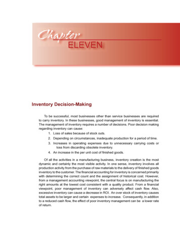
Management AccountingThe cost of various order sizes may be illustrated as follows:A 120,000P 100Order SizeOrder mber of orders120,0001242.41.71.331.091Total purchasingcost 12,000,000 1,200 400 240 170 133 109100Graphically, the cost of purchasing may be presented as follows:Figure 11-2 Graph of Total Purchasing CostTotal Purchasing Cost700060005000 0080000100000120000140000Order SizeAn order size of one unit per order results in a total and most likely unacceptablecost of 12,000,000. While an order size of 120,000 minimizes total purchasing costat 100, this order size is also most likely to be unacceptable, because of the highcarrying cost that would inevitably result due to the high average carrying cost thatwould invariably follow. The main point to observe is that as order size increases totalpurchasing cost decreases.There has been developed a tool that can determine the right order size and,therefore, the right number of times to purchase. This tool is commonly called anEOQ model. However, before this tool is mathematically introduced, it is necessaryto first discuss carrying costs.Carrying CostThe purchase of materials or the production of finished goods normally requires thatthe materials or finished goods be stored until used or sold. The storage of materials 201
202 CHAPTER ELEVEN Inventory Decision-Makingor finished goods obviously requires storage space. The greater the purchase lotat any given time, the greater is the storage space required. How long inventoryis stored varies directly with the rate at which it is used. In a restaurant where oneloaf of bread is purchased each time and a new loaf immediately purchased whenthe last loaf is used up, not much space would be require. On the other hand, if 144loaves are purchased at a time, then considerably more space would be required.Depending on the type of raw materials, some or all of the carrying costs could beincurred:1. Interest (a big order size requires an investment of money).2. Taxes (inventory is typically subject to a property tax).3. Insurance (inventory is always at risks like theft or fire or damage).4. Storage costs (inventory requires building space and is subject to thecosts associated with a building such as depreciation,5. Salary of storekeeper and helpers, if required.6. Spoilage.The basic principle of carrying inventory may be explained as follows: At a certainlevel of inventory (reorder point), a new order must be placed. The inventory at itsmaximum would be equal to the order size and at a minimum would be zero if nosafety stock is being carrying. Inventory is at a maximum when a new shipmentis received, and at its lowest moments before the new order arrives. As explainedearlier in this chapter, the inventory is not a constant amount and is best numericallydescribed as an average.Mathematically, total carrying cost is simply the average inventory for a period oftime times the cost of carrying a single unit of inventory: Therefore, mathematically,Order size––––––––––2Carrying cost IfESTCC-then:TCC x (Carrying cost per unit)represents order sizerepresents carrying cost per unitdenotes total carrying costE––––– (S)2(4)The cost of carrying inventory sizes may be illustrated the following table:A 120,000S 5.00Order SizeOrder verage 00Total carrying cost 2.50 25,000 75,000 125,000 175,000 225,000 275,000 300,000
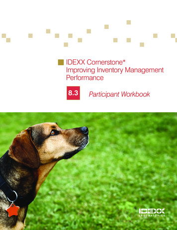
Management AccountingTotal carrying cost may be graphically illustrated as shown in figure 11.3:Figure 11-3 Graph of Total Carrying CostsTotal Carrying Cost350000300000250000 000150000Order SizeFigure 11-4 Graph of Total Inventory CostsEOQ Costs3500030000TotalPurchasingCost25000 20000TotalCarryingCost1500010000Total Cost50000010002000300040005000Order SizeAs order size increases, the total carrying cost increases. With an order size of1 unit carrying cost for the entire period is only 2.50. However, if the entire periodicneed for material is purchased one time, then the total carrying cost is 300,000, themaximum cost that can be incurred.Close observation of the above schedule reveals that as order size increases,total carrying cost also increases directly, just the opposite of total purchasing cost.A paradox then exists. Any attempt to minimize total purchasing cost, then increasestotal carrying cost and vice versus. The goal of inventory management becomesapparent: The goal should be then to minimize total purchasing cost and carrying costand not each cost separately. The two illustrations above concerning total purchasingcost and total carrying cost can now be combined as follows: 203
204 CHAPTER ELEVEN Inventory Decision-MakingOrder SizeOrder otal purchasingcost 12 M 1,200 400 240 170 133 109100Total carryingcost 2.50 25,000 75,000 125,000 175,000 225,000 275,000 300,000Total cost 12 m 26,200 75,400 125,240 175,170 225133 275,109 300,100It is apparent by observation that the order size of 10,000 shows the lowest totalcost of carrying and purchasing inventory. However, whether an order size of 10,000 isthe best order size has not been yet determined. An order size less than 10,000 mightresult in lower costs. This table may be graphically presented as shown above.From this graph the following observations may be made1. As order size increases, total purchasing cost decreases.2. As order size increases, total carrying cost increases3. Total cost is minimized where total purchasing cost equals total carryingcost.The observation that total cost of managing inventory can be minimized wheretotal purchasing cost equals total carrying cost allows us later to derive a formula fordetermining the best economic order size.EOQ FormulaEarlier total purchasing cost was defined as follows:TPC TPCAPE-A––– (P)Etotal purchasing costperiodic demand for materialcost of placing each orderorder sizeAlso, earlier total carrying cost was defined as follows:ETCC ––– (S)2S-carrying cost per unit of inventoryTotal cost can then be defined as follows:TCA –––– (P) EE–––– (S)2(5)
Management AccountingSince the best order size is where TPC TCC, we can mathematically solve forthe best order size as follows:AE–––– (P) ––––(S)E2Solving for E using basic algebra (see appendix to this chapter), we then get:E 2 A P(6)2Given the same values used previously as follows:A 120,000P 100S 5.00The order size that minimizes total cost then is :E 2 (120,000) ( 100) 5.00 2,191If this is the correct answer, then TPC should equal TCCTPC 120,000–––––––– ( 100) 5,4752,190.9TCC 2,190–––––––– ( 5) 5,4752Since TPC TCC, the best order size is 2,191 units.Illustrative ProblemThe L. K. Widget Company’s accountant presented the following informationbased on a cost analysis:Annual demand for materials (units)(A) 100Cost of placing an order(P) 10.00Cost per unit of carrying inventory(S) 5.00Based on the above information, economic order quantity may be computed asfollows: 205
206 CHAPTER ELEVEN Inventory Decision-MakingE 2 (100) ( 10) 5.00 20Using the same values given above, the following schedule may be prepared:Schedule of Costs of Carrying and Purchasing InventoryOrdersizeNumber chasingTotalCarryingTotalCost 1,000.00 2.50 1,002.501.0 200.00 12.50 212.5010.005.0 100.00 25.00 125.00156.677.5 66.67 37.50 104.17205.0010.0 50.00 50.00 100.00254.0012.5 40.00 62.50 102.50303.3015.0 33.00 75.00 108.00352.8517.5 28.50 87.50 116.00402.2220.0 22.00 100.00 122.00452.5022.5 25.00 112.50 137.50502.0025.0 20.00 125.00 145.00The most economical order size is 20. When order size is 20, then total carryingcost equals total purchasing costs and total cost is minimized at 100.The EOQ formula just discussed is based on several assumptions which if nottrue may result in values that are not helpful in making order size decisions. First, thisEOQ model requires an accurate estimate of demand under conditions of certainty.Extreme and frequent fluctuations in demand requires other approaches to the ordersize decision. Secondly, The EOQ model requires fairly accurate estimates of carryingand purchasing costs. Multiple products and numerous types of material for a singleproduct may make the computation of these costs very difficult.Making the Reorder Point DecisionWhen to reorder materials or parts is a decision that must be thoughtfullyconsidered. If the decision to reorder is made too late, then undesirable consequencessuch as stock outs and delays in production may happen. If the decision to reorderis made too soon, then unnecessary carrying costs will be incurred. The importantquestion then concerning reordering is: at what level of inventory should a new orderbe placed? Obviously, if inventory has reached zero, then the time to place an orderhas been missed. In formulating an answer to this question, a number of factors must
Management Accountingbe considered including:1. Lead time2. Average usage per day3. Desired safetyLead Time -Lead time is time between placing and order and receiving an order. Leadtime can vary greatly depending on a number of factors. It could be as little as a fewhours or as great as many months. Lead time can be affected by factors or conditionssuch as bad weather, strikes on the part of the supplier’s workers, production problemson the part of the suppliers, and unexpected problems in shipping. Because lead timecan vary with each order placed, the normal approach to developing a reorder pointis to use average lead time. When the variations are small, the use of average leadtime is workable. Lead time should be measured in terms of work days rather thancalendar days. If lead time is one day but the supplier of the material in questionis closed on Saturdays and Sundays, then a order placed on Friday might not bereceived until Tuesday of the next week. The problem of unpredictable variations inlead time can usually be solved by carrying safety stock.Average Usage per Day - It goes without saying that some level of materials inventoryis required to manufacture finished goods. A primary objective in the managementof the production process is to main a steady flow with minimal interruptions. Aconsistent daily production rate is highly desirable. If this goal is achieved, then theamount of material used each day is easily computed. Average usage per day willtend to be the same.To illustrate, if the production budget shows a planned production of 50,000widgets per year and each widget requires 10 units of material Z, then 500,000 unitsof material Z need to be purchased annually. If the year consists of 250 work days,then the following simple equation can be used to compute average usage per dayAnnual requirement for material500,000AUPD �––––––––––– –––––––– 2,000Work days250There is a connection between lead time and average usage per day. To avoida stock out, the level of inventory at the time an order is placed must be sufficient tolast until the new shipment arrives. This level of inventory, assuming no safety stock,can be computed simply by multiplying lead time times average usage per dayReorder point Lead time x Average Usage per Day (7)Safety Stock - Because both lead time and average usage per day can varysignificantly in the short run and to avoid stock outs during a critical time in theproduction process, it is normally desirable to carry some safety stock. The questionas to how much safety stock to carry is a difficult question to answer. If safety stock istoo small, then stock outs can still occur. If safety stock is to large, then unnecessarycarrying cost will be incurred. When average usage during lead time tends to bevolatile, safety stock models tend to be based on probability theory and requiresknowing the probability of different levels of demand during lead time. The use ofprobability models for safety stock is beyond the scope of this chapter. 207
208 CHAPTER ELEVEN Inventory Decision-MakingHowever, giving that a decision had been made regarding safety stock by whatevermethod, the equation for reorder point then becomes:Reorder point Lead time x Average Usage Per Day Safety Stock(8)Illustrative ProblemAssume the following:Annual demand for raw materialsNumber of work daysDesired safety stock levelLead time (days)25,0002501005Computing the reorder point requires, first of all, determining the average usageper day:25,000AUPD ––––––– 100250Reorder point then may be computed as follows:RP AUPD x Lead time safety stock (100 x 5) 100 600When inventory level becomes 600, then a new order should be placed.Theoretically, the new order should be received on the day the inventory reaches thesafety stock level of 100 units.Economic Order Quantity and Quantity DiscountsThe previous discussion on order size was based on the assumption that quantitydiscounts were not available. The EOQ formula as explained above is not able todetermine the most economic order size, given the availability of quantity discounts.Suppliers will often provide incentives to purchasers to buy in bigger quantities. Atypical discount schedule might look as follows:Quantity Discount Schedule for Material ZOrder SizePrice1-99 5.00100-199 4.00200-299 3.00300 2.50When quantity discounts are available, the basic EOQ formula can not be usedto directly solve for the best order size. However, it must be used on an iterative (trialand error) basis to find the best order size.When quantity discounts were not available, the cost of inventory itself,(purchases), was not relevant and could be ignored. However, because now theorder size affects the cost per unit, the total cost of inventory purchases must be
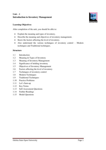
Management Accountingtaken into account. Without quantity discounts, the total cost of inventory purchasedremained the same regardless of order size. In order to solve for the best order size,the following equation must be used.AETC –––– (P) –––– (S) C(A)(9)E2The EOQ formula now has C(A), the total inventory purchase cost, as a cost element.When quantity discounts exists, the cost of inventory becomes relevant in the ordersize decision. C represents the cost of one unit of inventory. The other mathematicalsymbols have the same meaning as before:Erepresents order sizeSrepresents carrying cost per unitTCC denotes total carrying costTPC total purchasing costAperiodic demand for materialPcost of placing each orderEquation (9) above cannot be used to directly solve for order size (E). The reasonis that there are two unknowns: (1) order size and (2) cost per unit of inventory.Order size affects cost per unit and cost per unit affects order size. Because of thedependency of price on order size and order size on cost per unit of inventory, thetotal carrying cost curve and the total cost curve is now discontinuous as shown infigures 11-7 and 11-8.The trial and error procedure based on equation 9 that must be used is asfollows:Step 1Prepare a work sheet based on the total cost equation.Step 2Compute total cost at each price break, including an order size of oneunit.Step 3Determine the order size range which minimizes total cost. (In manycases the best order size is a price break quantity.)Figure 11.5 Total Purchasing Cost Figure 11.6 Total Carrying Cost Total Purchasing ,000150015001,0001,00050050050100150200Order Size250300Total Carrying Cost50100150200Order Size250300 209
210 CHAPTER ELEVEN Inventory Decision-MakingFigure 11-7 Cost of PurchasesFigure 11-8 Total Cost 50015001,0001,000500500Step 4100150200Order Size250Total Cost3,0002,50050Total Purchasing CostPurchasesTotal Carrying Cost30050100150200Order Size250Use the basic EOQ model to see if a better order size exists.IllustrationThe K. L. Widget Company may purchase Material Z at a quantity discount. Thecompany annually purchases 100 units. The cost of placing 1 order is 1. Carryingcost is 2.00 per unit. The following discount schedule is available:Quantity Discount Schedule for Material ZOrder SizePrice1-19 5.0020-29 4.9030-49 4.8050 4.70Work Sheet for Determining Best Order Size (Quantity Discounts hasingCost(A/E) PAverageInventory( E/2)TotalCarryingCost(E/2)SInventoryCostC( A)TotalCost1100 100.00.5 1.00 500 601.00205 5.0010 20.00 490 515.00303.3 3.3015 30.00 480 513.30502 2.0025 50.00 470 522.00EOQOrder size10 10.005 10.00 500 520.00300
Management AccountingStep 1Based on equation (2) the above work sheet was prepared.Step 2The price break quantities are 1, 20,30 and 50. For example, when 20units or more are ordered, then p
Inventory Decision-Making To be successful, most businesses other than service businesses are required to carry inventory. In these businesses, good management of inventory is essential. The management of inventory requires a number of decisions. Poor decision making regarding invent