Transcription
Miranda Holmes-CerfonApplied Stochastic Analysis, Spring 2019Lecture 2: Markov Chains (I)Readings Strongly recommended: Grimmett and Stirzaker (2001) 6.1, 6.4-6.6Optional: Hayes (2013) for a lively history and gentle introduction to Markov chains. Koralov and Sinai (2010) 5.1-5.5, pp.67-78 (more mathematical)A canonical reference on Markov chains is Norris (1997).We will begin by discussing Markov chains. In Lectures 2 & 3 we will discuss discrete-time Markov chains,and Lecture 4 will cover continuous-time Markov chains.2.1Setup and definitionsWe consider a discrete-time, discrete space stochastic process which we write as X(t) Xt , for t 0, 1, . . .The state space S is discrete, i.e. finite or countable, so we can let it be a set of integers, as in S {1, 2, . . . , N}or S {1, 2, . . .}.Definition. The process X(t) X0 , X1 , X2 , . . . is a discrete-time Markov chain if it satisfies the Markovproperty:P(Xn 1 s X0 x0 , X1 x1 , . . . , Xn xn ) P(Xn 1 s Xn xn ).(1)The quantities P(Xn 1 j Xn i) are called the transition probabilities. In general the transition probabilities are functions of i, j, n. It is convenient to write them aspi j (n) P(Xn 1 j Xn i) .(2)Definition. The transition matrix at time n is the matrix P(n) (pi j (n)), i.e. the (i, j)th element of P(n) ispi j (n).1 The transition matrix satisfies:(i) pi j (n) 0 i, j(ii) j pi j (n) 1 i(the entries are non-negative)(the rows sum to 1)Any matrix that satisfies (i), (ii) above is called a stochastic matrix. Hence, the transition matrix is a stochastic matrix.Exercise 2.1. Show that the transition probabilities satisfy (i), (ii) above.Exercise 2.2. Show that if X(t) is a discrete-time Markov chain, thenP(Xn s X0 x0 , X1 x1 , . . . , Xm xm ) P(Xn s Xm xm ) ,for any 0 m n. That is, the probabilities at the current time, depend only on the most recent known statein the past, even if it’s not exactly one step before.1We call it a matrix even if S .
Miranda Holmes-CerfonApplied Stochastic Analysis, Spring 2019Remark. Note that a “stochastic matrix” is not the same thing as a “random matrix”! Usually “random”can be substituted for “stochastic” but not here. A random matrix is a matrix whose entries are random.A stochastic matrix has completely deterministic entries. It probably gets its name because it is used todescribe a stochastic phenomenon, but this is an unfortunate accident of history.Definition. The Markov chain X(t) is time-homogeneous if P(Xn 1 j Xn i) P(X1 j X0 i), i.e. thetransition probabilities do not depend on time n. If this is the case, we write pi j P(X1 j X0 i) for theprobability to go from i to j in one step, and P (pi j ) for the transition matrix.We will only consider time-homogeneous Markov chains in this course, though we will occasionally remarkon how some results may be generalized to the time-inhomogeneous case.Examples1. Weather model Let Xn be the state of the weather on day n in New York, which we assume is eitherrainy or sunny. We could use a Markov chain as a crude model for how the weather evolves day-byday. The state space is S {rain, sun}. One transition matrix might beP sunrain sun0.80.4rain 0.20.6This says that if it is sunny today, then the chance it will be sunny tomorrow is 0.8, whereas if it israiny today, then the chance it will be sunny tomorrow is 0.4.One question you might be interested in is: what is the long-run fraction of sunny days in New York?2. Coin flipping Another two-state Markov chain is based on coin flips. Usually coin flips are used as thecanonical example of independent Bernoulli trials. However, Diaconis et al. (2007) studied sequencesof coin tosses empirically, and found that outcomes in a sequence of coin tosses are not independent.Rather, they are well-modelled by a Markov chain with the following transition probabilities:P headstails heads0.510.49tails 0.490.51This shows that if you throw a Heads on your first toss, there is a very slightly higher chance ofthrowing heads on your second, and similarly for Tails.3. Random walk on the line Suppose we perform a walk on the integers, starting at 0. At each time wemove right or left by one unit, with probability 1/2 each. This gives a Markov chain, which can beconstructed explicitly asnXn ξ j,ξ j 1with probabilityj 11each,2The transition probabilities are1pi,i 1 ,21pi,i 1 ,22pi, j 0( j 6 i 1).ξi i.i.d.
Miranda Holmes-CerfonApplied Stochastic Analysis, Spring 2019The state space is S {. . . , 1, 0, 1, . . .}, which is countably infinite.There are various things we might want to know about this random walk – for example, what is theprobability of ever reaching level 10, i.e. what is the probability that Xn 10 for some n? And, whatis the average number of steps it takes to do this? Or, what is the average distance to the origin, orsquared distance to the origin, as a function of time? Or, how does the probability distribution of thewalker evolve? We will see how to answer all of these questions.4. Gambler’s ruin This is a modification of a random walk on a line, designed to model certain gamblingsituations. A gambler plays a game where she either wins 1 with probability p, or loses 1 withprobability 1-p. The gambler starts with k , and the game stops when she either loses all her money,or reaches a total of n .The state space of this Markov chain is S {0, 1, . . . , n} and the transition matrix has entries pif j i 1, 0 i n, 1 p if j i 1, 0 i n,Pi j 1if i j 0, or i j n, 0otherwise.For example, when n 5 and p 0.4 the transition matrix is01P 23450 1 0.6 0 0 001000.6000200.400.6003000.400.6040000.40050 0 0 0 0.41Questions of interest might be: what is the probability the gambler wins or loses? Or, after a givennumber of games m, what is the average amount of money the gambler has?5. Independent, identically distribute (i.i.d.) random variables A sequence of i.i.d. random variables isa Markov chain, albeit a somewhat trivial one. Suppose we have a discrete random variable X takingvalues in S {1, 2, . . . , k} with probability P(X i) pi . If we generate an i.i.d. sequence X0 , X1 , . . .of random variables with this probability mass function, then it is a Markov chain with transitionmatrix12 ··· k1 p1 p2 · · · pk 2 p1 p2 · · · pk P . . . .k p1 p2 · · · pk6. Random walk on a graph (undirected, unweighted) Suppose we have a graph (a set of vertices andedge connecting them.) We can perform a random walk on the graph as follows: if we are at node i,3
Miranda Holmes-CerfonApplied Stochastic Analysis, Spring 2019choose an edge uniformly at random from the set of edges leading out of the node, and move alongthe edge to the node at the edge. Then repeat. If there are N nodes labelled by consecutive integersthen this is a Markov chain on state space S {1, 2, . . . , N}.Here is are a couple of examples:213321454The corresponding transition matrices are:11 01P 2 133 34 023121313121300140 0 1 12P 345301 0 12 0 0122301212012000012400120051 20 0 1 2127. Random walk on a graph (weighted, directed)Every Markov chain can be represented as a random walk on a weighted, directed graph. A weightedgraph is one where each edge has a positive real number assigned to it, its “weight,” and the randomwalker chooses an edge from the set of available edges, in proportion to each edge’s weight. In adirected graph each edge also has a direction, and a walker can only move in that direction. Here is anexample:A23112BC44
Miranda Holmes-CerfonApplied Stochastic Analysis, Spring 2019The corresponding transition matrix is: AA 0P B 15C 36B1026C 04 516In fact, such a directed graph forms the foundation for Google’s Page Rank algorithm, which hasrevolutionized internet searches. The earliest and best-known version of Page Rank constructs a directed graph of the internet, where nodes are webpages and there is a directed edge from webpage Ato webpage B if A contains a link to B. Page Rank assumes an internet surfer clicks follows links atrandom, and ranks pages according to the long-time average fraction of time that the surfer spends oneach page.8. Ehrenfest model of diffusion Consider a container with a membrane in the middle, and m particles distributed in some way between the left and right sides. At each step, pick one particle atrandom and move it to the other side. Let Xn # of particles inthe left side at time n. Then Xn is a Markov chain, with transitionprobabilities pi,i 1 1 mi , pi,i 1 mi .9. Card shuffling Shuffling a pack of cards can be modeled as a Markov chain. The state space S isthe set of permutations of {1, 2, . . . , 52}. A shuffle takes one permutation σ S, and outputs anotherpermutation σ 0 S with a certain probability.Perhaps the simplest model is the top-to-random shuffle: at each step, take a card from the top of thedeck, and put it back in at a random location. The transition matrix has elements 1 52 if σ 0 is obtained by taking an item in σ0P(X1 σ X0 σ ) and moving it to the top, 0 otherwise.One can also model more complicated shuffles, such as the riffle shuffle. While the state space isenormous ( S 52!) so you would not want to write down the whole transition matrix, one can stillanalyze these models using other techniques, from analysis and probability theory. Various authorshave proven results about the number of shuffles needed to make the deck “close to random”. Forexample, it takes seven riffle shuffles to get close to random, but it takes 11 or 12 to get so closethat a gambler in a casino cannot exploit the deviations from randomness to win a typical game. Seethe online essay Austin (line) for an accessible introduction to these ideas, and Aldous and Diaconis(1986) for the mathematical proofs. (I first learned about this phenomenon in the beautiful Proofsfrom the Book, by Aigner and Ziegler.)10. Autoregressive model of order k (AR(k)) Given constants a1 , . . . , ak R, let Yn a1Yn 1 a2Yn 2 . . . akYn k Wn , where Wn are i.i.d. random variables.5
Miranda Holmes-CerfonApplied Stochastic Analysis, Spring 2019This process is not Markov, because it depends on the past k timesteps. However, we can form aMarkov process by defining Xn (Yn ,Yn 1 , . . . ,Yn k 1 )T . ThenXn AXn 1 Wn , a1 1where A 0···a201···············1 ak0 , and Wn (Wn , 0, . . . , 0)T .0 011. Language, and history of the Markov chain Markov chains were first invented by Andrei Markov toanalyze the distribution of letters in Russian poetry (Hayes (2013)).2 He meticulously constructed alist of the frequencies of vowel consonant pairs in the first 20,000 letters of Pushkin’s poem-novelEugene Onegin, and constructed a transition matrix from this data. His transition matrix was:vowelP consonant vowel0.1750.526consonant 0.8250.474He showed that from this matrix one can calculate the average number of vowels and consonants.When he realized how powerful this idea was, he spent several years developing tools to analyze theproperties of such random processes with memory.Just for fun, here’s an example (from Hayes (2013)) based on Markov’s original example, to showhow Markov chains can be used to generate realistic-looking text. In each of these excerpts, a Markovchain was constructed by considering the frequencies of strings of k letters from the English translationof the novel Eugene Onegin by Pushkin, for k 1, 3, 5, 7, and was then run from a randomly-generatedinitial condition. You can see that when k 3, there are English-looking syllables, when k 5 thereare English-looking words, and when k 7 the words themselves almost fit together coherently.2 Actually, he invented Markov chains to disprove a colleague’s statement that the Law of Large Numbers can only hold for independent sequences of random variables, and he illustrated his new ideas on this vowel/consonant example.6
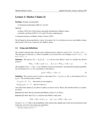
Miranda Holmes-CerfonApplied Stochastic Analysis, Spring 201912. Markov chains in applications. Markov chains arise in a great many modern applications. Here is anexample, from Rogers et al. (2013), where the configuration space of two DNA-coated colloids wasmodelled as a two-state Markov chain, with states “bound” and “unbound,” depending on whether thedistance between the particles was small or large:Some other examples of applications that use Markov chains include: models of physical processes– rainfall from day-to-day– neural networks– population dynamics– lineups, e.g. in grocery stores, computer servers, telephone call centers, etc.– chemical reactions– protein folding– baseball statistics discretize a continuous system7
Miranda Holmes-CerfonApplied Stochastic Analysis, Spring 2019 sampling from high-dimensional systems, e.g. Markov-Chain Monte-Carlo data/network analysis– clustering– speech recognition– PageRank algorithm in Google’s search engine.2.2Evolution of probabilityGiven a Markov chain with transition probabilities P and initial condition X0 i, we know how to calculatethe probability distribution of X1 ; indeed, this is given directly from the transition probabilities. The naturalquestion to ask next is: what is the distribution at later times? That is, we would like to know the n-steptransition probabilities P(n) , defined by(n)Pi j P(Xn j X0 i).(3)For example, for n 2, we have thatP(X2 j X0 i) P(X2 j X1 k, X0 i)P(X1 k X0 i)Law of Total Probabilityk P(X2 j X1 k)P(X1 k X0 i)Markov Propertyk Pk j Piktime-homogeneityk (P2 )i jThat is, the two-step transition matrix is P(2) P2 .This generalizes:Theorem. Let X0 , X1 , . . . be a time-homogeneous Markov chain with transition probabilities P. The n-steptransition probabilities are P(n) Pn , i.e.P(Xn j X0 i) (Pn )i j .(4)To make the notation cleaner we will write (Pn )i j Pinj . Note that this does not equal (Pi j )n .Exercise 2.3. Prove this theorem. Hint: use induction.A more general equation relating the transition probabilities, that holds even in the time-inhomogeneouscase, is:Chapman-Kolmogorov Equation.P(Xn j X0 i) P(Xn j Xm k)P(Xm k X0 i).k8(5)
Miranda Holmes-CerfonApplied Stochastic Analysis, Spring 2019Proof.P(Xn j X0 i) P(Xn j, Xm k X0 i)Law of Total Probabilityk P(Xn j Xm k, X0 i)P(Xm k X0 i) P(A B C) P(A B C)P(B C)k RHSby Markov property (see Ex.(2.2))Remark. In the time-homogeneous case, the CK equations may be written more compactly asPm n Pm Pn .(6)When S , we understand a power such as P2 to mean the infinite sum (P2 )i j k Pk j Pik .Remark. All Markov Processes satisfy a form of Chapman-Kolmogorov equations, from which many otherequations can be derived. However, not all processes which satisfy Chapman-Kolmogorov equations, areMarkov processes. See Grimmett and Stirzaker (2001), p.218 Example 14 for an example.Now suppose we don’t know the initial condition of the Markov chain, but rather we know the probabilitydistribution of the initial condition. That is, X0 is a random variable with distribution P(X0 i) ai . Wewill write this asX0 α (0) (a1 , a2 , . . . , ).Here α (0) is a row vector representing the pmf of the initial condition. It is important that it is a row vector– this is the convention, which both simplifies notation and makes it easier to generalize to continuous-stateMarkov processes.We would like to calculate the distribution of Xn , which we write as a row vector α (n) :(n)αi P(Xn i).Let’s calculate α (n 1) , assuming we know α (n) .(n 1)αj P(Xn 1 j Xn i)P(Xn i)Law Of Total Probabilityi(n)time-homogeneity and defn of α (n) . Pi j αiiWe obtain:Forward Kolmogorov Equation. (for a time-homogeneous, discrete-time Markov Chain)α (n 1) α (n) P.(7)This equation shows how to evolve the probability in time. The solution is clearly α (n) α (0) Pn , which youcould also show directly from the n-step transition probabilities.Exercise 2.4. Do this! Show that (7) holds, directly from the formula for the n-step transition probabilities.9
Miranda Holmes-CerfonApplied Stochastic Analysis, Spring 2019Therefore, if we know the initial probability distribution α (0) , then we can find the distribution at any latertime using powers of the matrix P.Now consider what happens if we ask for the expected value of some function of the state of the Markovchain, such as EXn2 , EXn3 , E Xn , etc. Can we derive an evolution equation for this quantity?Let f : S R be a function defined on state space, and let(n)ui Ei f (Xn ) E[ f (Xn ) X0 i].(8)You should think of u(n) as a column vector; again this is a convention whose convenience will become moretransparent later in the course. Then u(n) evolves in time as:Backward Kolmogorov Equation. (for a time-homogeneous, discrete-time Markov Chain)u(n 1) Pu(n) ,u(0) (i) f (i) i S.(9)Proof. We haveu(n 1) (i) f ( j)P(Xn 1 j X0 i)definition of expectationj f ( j)P(Xn 1 j X1 k, X0 i)P(X1 k X0 i)j f ( j)P(Xn 1 j X1 k)P(X1 k X0 i)jtime-homogeneityk f ( j)Pknj PikkMarkov propertyk f ( j)Pknj PikjLoTPkswitch order of summationj u(n) (k)Pikdefinition of u(n)k (Pu)iWe can switch the order of summation above, provided we assume that Ei f (Xn ) for each i and eachn.This proof illustrates a technique sometimes known as first-step analysis, where one conditions on the firststep of the Markov chain and uses the Law of Total Probability. Of course, you could also derive thisequation more directly from the n-step transition probabilities.Exercise 2.5. Do this! Derive (9) directly from the formula for the n-step transition probabilities.Remark. What is so backward about the backward equation? It gets its name from the fact that it can be usedto describe how conditional expectations propagate backwards in time. To see this, suppose that instead of(8), which computes the expectation of a function after a certain number of steps has passed, we choose afixed time T and compute the expectation at that time, given an earlier starting position. That is, for eachn T , define a column vector u(n) with components(n)ui E[ f (XT ) Xn i] .10(10)
Miranda Holmes-CerfonApplied Stochastic Analysis, Spring 2019Such a quantity is studied a lot in financial applications, where, say, Xn is the price of a stock at time n, f is avalue function representing the value of an option to sell, T might be a time at which you decide (in advance)to sell a stock, and quantities of the form (10) above would represent your expected payout, conditional onbeing in state i at time n. Then, the vector u(n) evolves according to(T )u(n) Pu(n 1) ,ui f (i) i S.(11)Therefore you find u(n) by evolving it backwards in time – you are given a final condition at time T , and youcan solve for un at all earlier times n T .Interestingly, (11) holds even when the chain is not time-homogeneous, provided that P in (11) is replacedby P(n), the transition probabilities starting at time n. This same statement is not true for (9).Exercise 2.6. Show (11), and argue it holds even when the Markov chain is not time-homogeneous.2.2.1Evolution of the full transition probabilities*Another approach to the forward/backward equations is to define a function P( j,t i, s) to be the transitionprobability to be in state j at time t, given the system started in state i at time s, i.e.P( j,t i, s) P(Xt j Xs i).(12)One can then derive equations for how P( j,t i, s) evolves in t and s. For evolution in t (forward in time) wehave, from the Chapman-Kolmogorov equations,P( j,t 1 i, s) P(k,t i, s)P( j,t 1 k,t).(13)kFor evolution in s (backward in time) we have, again from the Chapman-Kolmogorov equations,P( j,t i, s) P( j,t k, s 1)P(k, s 1 i, s).(14)kThese are general versions of the forward and backward equations, respectively. They hold regardless ofwhether the chain is time-homogeneous or not. From them, we can derive the time-inhomogeneous versionsof the forward and backward equations (7), (9).To derive the time-inhomogeneous forward equation, notice that the probability distribution at time t, α (t) ,(t)(0)has components α j i P( j,t i, 0)αi . Therefore, multiplying (13) by α (0) on the left (contracting it withindex i) and letting s 0, we obtain(t 1)αj(t) αk P( j,t 1 k,t) (t)α (t 1) α (t) Pk j .(15)k(s)To derive the time-inhomogeneous backward equation, let f : S R, and let ui E[ f (Xt ) Xs i] (recall(s)(8),(10).) Notice that ui k f (k)P(k,t i, s), so multiplying (14) by the column vector f on the right(contracting it with index j) gives(s)(s 1) ui P(k, s 1 i, s)ukk11(s)u(s) Pi j u(s 1) .(16)
Miranda Holmes-Cerfon2.3Applied Stochastic Analysis, Spring 2019Long-time behaviour and stationary distributionSuppose we take a Markov chain and let it run for a long time. What happens? Clearly the chain itself doesnot converge to anything, because it is continually jumping around, but the probability distribution might.Before getting into the theory, let’s look at some examples.Consider the two-state weather model from section 2.1, example 1. Suppose it is raining today. Whatis the probability distribution for the weather in the future? We calculate this from the n-step transitionprobabilities 330.3333It seems like the probability distribution is converging to something. After 12 days, the distribution doesn’tchange, to 4 digits. You can check that the distribution it converges to does not depend on the initial condition. For example, if we start with a sunny day, α (0) (1, 0), then α (10) (0.6666, 0.3334), α (11) (0.6666, 0.3334), α (12) (0.6667, 0.3333). In fact, this example is simple enough that you could workout the n-step transition probabilities for any initial condition analytically, and show they converge to(2/3, 1/3).Exercise 2.7. Do this! (Hint: calculate eigenvalues of the transition matrix.)Does the probability always converge? Let’s look at another example. Consider a Markov chain on statespace {0, 1} with transition matrix 0 1P .1 0Suppose the random walker starts at state 0. Its distribution at time n is:12
Miranda Holmes-CerfonApplied Stochastic Analysis, Spring 2019n0123456.P(0)1010101.P(1)0101010.You can see the pattern. Clearly the distribution doesn’t converge. Yet, if we start with initial distirbutionα (0) (0.5, 0.5), then we obtainn012.P(0)0.50.50.5.P(1)0.50.50.5.The distribution never changes!2.3.1Limiting and stationary distributionsIn applications we are often interested in the long-term probability of visiting each state.Definition. Consider a time-homogeneous Markov chain with transition matrix P. A row vector λ is alimiting distribution if λi 0, j λ j 1 (so that λ is a probability distribution), and if, for every i,lim (Pn )i j λ j j S.n In other words, λ1 λ1 Pn λ1 .λ2λ2λ2. . . . . . . .λ3λ3λ3.as n .Exercise 2.8. Show that, if S , then λ is a limiting distribution if and only if the definition limn αPn λ for any initial probability distribution α.As we saw in the earlier examples, a limiting distribution doesn’t have to exist. If it exists, it must be unique.What happens if we start the chain in the limiting distribution? Let’s calculate the distribution α (1) at thenext step of the chain, assuming initial distribution α (0) λ . For simplicity, we will assume a finite statespace, S , which lets us interchange the sum and the limit in the calculations below. Choose any i, andcalculate, from (7), (writing Ai,· for the row vector corresponding to the ith row of matrix A): α (1) λ P lim Pi,·n P lim Pi,·n 1 λ .n n 13
Miranda Holmes-CerfonApplied Stochastic Analysis, Spring 2019Therefore if we start the chain in the limiting distribution, its distribution remains there forever. This motivates the following definition:Definition. Given a Markov chain with transition matrix P, a stationary distribution is a probability distribution π which satisfiesπ πP π j πi Pi j j.(17)iThis says that that if we start with distribution π and run the Markov chain, the distribution will not change.That is why it is called “stationary.” In other words, if X0 π, then X1 π, X2 π, etc.Remark. Other synonyms you might hear for stationary distribution include invariant measure, invariantdistribution, steady-state probability, equilibrium probability or equilibrium distribution (the latter two arefrom physics.).In applications we want to know the limiting distribution, but it is usually far easier to calculate the stationarydistribution, because it is obtained by solving a system of linear equations. Therefore we will restrict ourfocus to the stationary distribution. Some questions we might ask about π include:(i) Does it exist?(ii) Is it unique?(iii) When is it a limiting distribution, i.e. when does an arbitrary distribution converge to it?For (iii), we saw that a limiting distribution is a stationary distribution, but the converse is not always true.Indeed, in our second example, you can calculate that a stationary distribution is π (0.5, 0.5), but this isnot a limiting distribution. What are the conditions that guarantee a stationary distribution is also the limitingdistribution?This is the subject of a rich body of work on the limiting behaviour of Markov chains. We will not go deeplyinto the results, but will briefly survey a couple of the major theorems.2.3.2A limit theorem or twoDefinition. A matrix A is positive if it has all positive entries: Ai j 0 for all i, j. In these notes we will writeA 0 when A is positive.Remark. This is not the same as being positive-definite!Definition. A stochastic matrix is regular if there exists some s 0 such that Ps is positive, i.e. the s-steptransition probabilities are positive for all i, j: (Ps )i j 0 i, j.Remark. Some books call such a matrix primitive. The text Koralov and Sinai (2010)) calls it ergodic (whenthe state space is finite), though usually this word is reserved for something slightly different.This means that there is a time s such that, no matter where you start, there is a non-zero probability of beingat any other state.Theorem (Ergodic Theorem for Markov Chains, (one version)). Assume a Markov Chain is regular andhas a finite state space with size N. Then there exists a unique stationary probability distribution π (π1 , . . . , πN ), with π j 0 j. The n-step transition probabilities converge to π: that is, limn Pinj π j .14
Miranda Holmes-CerfonApplied Stochastic Analysis, Spring 2019Remark. The name of this theorem comes from Koralov and Sinai (2010); it may not be universal. Thereare many meanings of the word “ergodic”; we will see several variants throughout this course.Remark. For a Markov chain with an infinite state space, the Ergodic theorem holds provided the chain isirreducible (see below), aperiodic (see below), and all states have finite expected return times (ask instructor– this condition is always true for finite irreducible chains.) For a proof, see Dobrow (2016), section 3.10.Proof. This is a sketch, see Koralov and Sinai (2010) p.72 for all the details.– Define a metric d(µ 0 , µ 00 ) 21 Ni 1 µi0 µi00 on the space of probability distributions. It can be shownthat d is a metric, and the space of distributions is complete.– Show (*) d(µ 0 Q, µ 00 Q) (1 α)d(µ 0 , µ 00 ), where α mini, j Qi j and Q is a stochastic matrix.– Show that µ (0) , µ (0) P, µ (0) P2 , . . . is a Cauchy sequence. Therefore it converges, so let π limn µ (n) .– Show that π is unique: let π1 , π2 be two distributions such that πi π1 P. Then d(π1 , π2 ) d(π1 Ps , π2 Ps ) (1 α)d(π1 , π2 ) by (*). Therefore d(π1 , π2 ) 0.– Let µ (0) be the probability distribution which is concentrated at point i. Then µ (0) Pn is the probability(n)(n)distribution (pi j ). Therefore, limn pi j π j .Remark. This shows that d(µ (0) Pn , π) (1 α) 1 β n , with β (1 α)1/s 1. Therefore the rate ofconvergence to the stationary distribution is exponential.There is also a version of the Law of Large Numbers.Theorem (Law of large numbers for a regular Markov chain). Let π be the stationary distribution of a(n)regular Markov chain, and let νi be the number of occurences of state i in after n time steps of the(n)chain, i.e. among the values of X0 , X1 , . . . , Xn . Let νi j be the number of values of k, 1 k n, for whichXk 1 i, Xk j. Then for any ε 0,(n)νlim P( i πi ε) 0n n(n)lim P( n νi jn πi pi j ε) 0Proof. For a proof, see Koralov and Sinai (2010), p. 74.Remark. This implies that the long-time average of any function of a regular Markov chain,approaches the average with respect to the stationary distribution, Eπ f (X).1n ni 1 f (Xn ),This theorem can be weakened slightly by allowing for Markov chains with some kind of periodicity. Weneed to consider a chain which can move between any two states (i, j), but not necessarily at a time s that isthe same for all pairs.Definition. A stochastic matrix is irreducible if, for every pair (i, j) there exists an s 0 such that (Ps )i j 0.15
Miranda Holmes-CerfonApplied Stochastic Analysis, Spring 2019There are limit theorems for irreducible chains, with slightly weaker conditions. Irreducible chains also havea unique stationary distribution – this follows from the Perron-Frobenius Theorem (see below.) However, itis not true that an arbitrary distribution converges to it; rather, we have that µ (0) P̄(n) π as n , whereP̄(n) 1n nk 1 Pk . This means that the average distribution converges. We need to form the average, becausethere may be a built-in periodicity, as in the chain in the second example. In this case P2n I, and P2n 1 P,
rainy or sunny. We could use a Markov chain as a crude model for how the weather evolves day-by-day. The state space is S frain;sung. One transition matrix might be P sun rain sun 0:8 0:2 rain 0:4 0:6 This says that if