Transcription
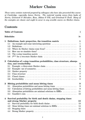
Markov ChainsThese notes contain material prepared by colleagues who have also presented this courseat Cambridge, especially James Norris. The material mainly comes from books ofNorris, Grimmett & Stirzaker, Ross, Aldous & Fill, and Grinstead & Snell. Many ofthe examples are classic and ought to occur in any sensible course on Markov chains.ContentsTable of ContentsiSchedulesiv1 Definitions, basic properties, the transition1.1 An example and some interesting questions1.2 Definitions . . . . . . . . . . . . . . . . . . .1.3 Where do Markov chains come from? . . . .1.4 How can we simulate them? . . . . . . . . .1.5 The n-step transition matrix . . . . . . . .1.6 P (n) for a two-state Markov chain . . . . .matrix. . . . . . . . . . . . . . . . . . . . . . . . .11233342 Calculation of n-step transition probabilities, class structure, absorption, and irreducibility52.1 Example: a three-state Markov chain . . . . . . . . . . . . . . . . . . . .52.2 Example: use of symmetry . . . . . . . . . . . . . . . . . . . . . . . . . .62.3 Markov property . . . . . . . . . . . . . . . . . . . . . . . . . . . . . . .62.4 Class structure . . . . . . . . . . . . . . . . . . . . . . . . . . . . . . . .72.5 Closed classes . . . . . . . . . . . . . . . . . . . . . . . . . . . . . . . . .82.6 Irreducibility . . . . . . . . . . . . . . . . . . . . . . . . . . . . . . . . .83 Hitting probabilities and mean hitting times3.1 Absorption probabilities and mean hitting times . . . . . .3.2 Calculation of hitting probabilities and mean hitting times .3.3 Absorption probabilities are minimal solutions to RHEs . .3.4 Gambler’s ruin . . . . . . . . . . . . . . . . . . . . . . . . .4 Survival probability for birth and death chains, stoppingand strong Markov property4.1 Survival probability for birth death chains . . . . . . . . . .4.2 Mean hitting times are minimal solutions to RHEs . . . . .4.3 Stopping times . . . . . . . . . . . . . . . . . . . . . . . . .4.4 Strong Markov property . . . . . . . . . . . . . . . . . . . .i.9991112.1313141515times.
5 Recurrence and transience5.1 Recurrence and transience . . . . . . . . . . . . . . . . . . . . . . . . . .5.2 Equivalence of recurrence and certainty of return . . . . . . . . . . . . .5.3 Equivalence of transience and summability of n-step transition probabilities5.4 Recurrence as a class property . . . . . . . . . . . . . . . . . . . . . . .5.5 Relation with closed classes . . . . . . . . . . . . . . . . . . . . . . . . .1717171818196 Random walks in dimensions one, two and three6.1 Simple random walk on Z . . . . . . . . . . . . . .6.2 Simple symmetric random walk on Z2 . . . . . . .6.3 Simple symmetric random walk on Z3 . . . . . . .6.4 *A continuized analysis of random walk on Z3 * . .6.5 *Feasibility of wind instruments* . . . . . . . . . .7 Invariant distributions7.1 Examples of invariant distributions . . . . . . .7.2 Notation . . . . . . . . . . . . . . . . . . . . . .7.3 What does an invariant measure or distribution7.4 Invariant distribution is the solution to LHEs .7.5 Stationary distributions . . . . . . . . . . . . .7.6 Equilibrium distributions . . . . . . . . . . . .212122232424. . . . . . . . .tell us?. . . . . . . . . . . . .25252526262828.8 Existence and uniqueness of invariant distribution, mean returnpositive and null recurrence8.1 Existence and uniqueness up to constant multiples . . . . . . . . .8.2 Mean return time, positive and null recurrence . . . . . . . . . . .8.3 Random surfer . . . . . . . . . . . . . . . . . . . . . . . . . . . . .9 Convergence to equilibrium for ergodic chains9.1 Equivalence of positive recurrence and the existence of an invarianttribution . . . . . . . . . . . . . . . . . . . . . . . . . . . . . . . . .9.2 Aperiodic chains . . . . . . . . . . . . . . . . . . . . . . . . . . . .9.3 Convergence to equilibrium *and proof by coupling* . . . . . . . .time,. . . . . . .2929313233dis. . . . . . .33343510 Long-run proportion of time spent in given state10.1 Ergodic theorem . . . . . . . . . . . . . . . . . . . . . . . . . . . . . . .10.2 *Kemeny’s constant and the random target lemma* . . . . . . . . . . .37373911 Time reversal, detailed balance, reversibility, random walk on a graph11.1 Time reversal . . . . . . . . . . . . . . . . . . . . . . . . . . . . . . . . .11.2 Detailed balance . . . . . . . . . . . . . . . . . . . . . . . . . . . . . . .11.3 Reversibility . . . . . . . . . . . . . . . . . . . . . . . . . . . . . . . . . .11.4 Random walk on a graph . . . . . . . . . . . . . . . . . . . . . . . . . .4141424343ii
12 Concluding problems and recommendations for12.1 Reversibility and Ehrenfest’s urn model . . . . .12.2 Reversibility and the M/M/1 queue . . . . . . .12.3 *The probabilistic abacus* . . . . . . . . . . . . .12.4 *Random walks and electrical networks* . . . . .12.5 Probability courses in Part II . . . . . . . . . . .further. . . . . . . . . . . . . . . . . . . . .study. . . . . . . . . . . . . . . .454546474750Appendix51A Probability spaces51B Historical notes52C The probabilistic abacus for absorbing chains53Index56Topics marked * * are non-examinable. Furthermore, only Appendix A is examinable.Richard Weber, October 2011iii
SchedulesDefinition and basic properties, the transition matrix. Calculation of n-step transitionprobabilities. Communicating classes, closed classes, absorption, irreducibility. Calculation of hitting probabilities and mean hitting times; survival probability for birth anddeath chains. Stopping times and statement of the strong Markov property. [5]Recurrence and transience; equivalence of transience and summability of n-steptransition probabilities; equivalence of recurrence and certainty of return. Recurrenceas a class property, relation with closed classes. Simple random walks in dimensionsone, two and three. [3]Invariant distributions, statement of existence and uniqueness up to constant multiples. Mean return time, positive recurrence; equivalence of positive recurrence andthe existence of an invariant distribution. Convergence to equilibrium for irreducible,positive recurrent, aperiodic chains *and proof by coupling*. Long-run proportion oftime spent in given state. [3]Time reversal, detailed balance, reversibility; random walk on a graph. [1]Learning outcomesA Markov process is a random process for which the future (the next step) dependsonly on the present state; it has no memory of how the present state was reached. Atypical example is a random walk (in two dimensions, the drunkards walk). The courseis concerned with Markov chains in discrete time, including periodicity and recurrence.For example, a random walk on a lattice of integers returns to the initial positionwith probability one in one or two dimensions, but in three or more dimensions theprobability of recurrence in zero. Some Markov chains settle down to an equilibriumstate and these are the next topic in the course. The material in this course will beessential if you plan to take any of the applicable courses in Part II. Learning outcomesBy the end of this course, you should: understand the notion of a discrete-time Markov chain and be familiar with boththe finite state-space case and some simple infinite state-space cases, such asrandom walks and birth-and-death chains; know how to compute for simple examples the n-step transition probabilities,hitting probabilities, expected hitting times and invariant distribution; understand the notions of recurrence and transience, and the stronger notion ofpositive recurrence; understand the notion of time-reversibility and the role of the detailed balanceequations; know under what conditions a Markov chain will converge to equilibrium in longtime; be able to calculate the long-run proportion of time spent in a given state.iv
1Definitions, basic properties, the transition matrixMarkov chains were introduced in 1906 by Andrei Andreyevich Markov (1856–1922)and were named in his honor.1.1An example and some interesting questionsExample 1.1. A frog hops about on 7 lily pads. The numbers next to arrows show theprobabilities with which, at the next jump, he jumps to a neighbouring lily pad (andwhen out-going probabilities sum to less than 1 he stays where he is with the remainingprobability). 1112121271212123121414451216 0100000 0 1 2 P 0 0 0 0120000000121214121400000120010000000 0 0 0 1 2 0 10There are 7 ‘states’ (lily pads). In matrix P the element p57 ( 1/2) is the probabilitythat, when starting in state 5, the next jump takes the frog to state 7. We would liketo know where do we go, how long does it take to get there, and what happens in thelong run? Specifically:(a) Starting in state 1, what is the probability that we are still in state 1 after 3(3)(5)steps? (p11 1/4) after 5 steps? (p11 3/16) or after 1000 steps? ( 1/5 as(n)limn p11 1/5)(b) Starting in state 4, what is the probability that we ever reach state 7? (1/3)(c) Starting in state 4, how long on average does it take to reach either 3 or 7? (11/3)(d) Starting in state 2, what is the long-run proportion of time spent in state 3? (2/5)Markov chains models/methods are useful in answering questions such as: How longdoes it take to shuffle deck of cards? How likely is a queue to overflow its buffer? Howlong does it take for a knight making random moves on a chessboard to return to hisinitial square (answer 168, if starting in a corner, 42 if starting near the centre). Whatdo the hyperlinks between web pages say about their relative popularities?1
1.2DefinitionsLet I be a countable set, {i, j, k, . . . }. Each i I is called a state and I is called thestate-space.We work in a probability space (Ω, F , P ). Here Ω is a set of outcomes, F is aset of subsets of Ω, and for A F , P (A) is the probability of A (see Appendix A).The object of our study is a sequence of random variables X0 , X1 , . . . (taking valuesin I) whose joint distribution is determined by simple rules. Recall that a randomvariable X with values in I is a function X : Ω I.A row vector λ (λi : i I) is called a measure if λi 0 for all i.PIf i λi 1 then it is a distribution (or probability measure). We start with aninitial distribution over I, specified by {λi : i I} such that 0 λi 1 for all i andPi I λi 1.The special case that with probability 1 we start in state i is denoted λ δi (0, . . . , 1, . . . , 0).We also have a transition matrix P (pij : i, j I) with pij 0 for all i, j.PIt is a stochastic matrix, meaning that pij 0 for all i, j I and j I pij 1(i.e. each row of P is a distribution over I).Definition 1.2. We say that (Xn )n 0 is a Markov chain with initial distribution λand transition matrix P if for all n 0 and i0 , . . . , in 1 I,(i) P (X0 i0 ) λi0 ;(ii) P (Xn 1 in 1 X0 i0 , . . . , Xn in ) P (Xn 1 in 1 Xn in ) pin in 1 .For short, we say (Xn )n 0 is Markov (λ, P ). Checking conditions (i) and (ii) isusually the most helpful way to determine whether or not a given random process(Xn )n 0 is a Markov chain. However, it can also be helpful to have the alternativedescription which is provided by the following theorem.Theorem 1.3. (Xn )n 0 is Markov(λ, P ) if and only if for all n 0 and i0 , . . . , in I,P (X0 i0 , . . . , Xn in ) λi0 pi0 i1 · · · pin 1 in .(1.1)Proof. Suppose (Xn )n 0 is Markov(λ, P ). ThenP (X0 i0 , . . . , Xn in ) P (Xn in X0 i0 , . . . , Xn 1 in 1 )P (X0 i0 , . . . , Xn 1 in 1 ) P (X0 i0 )P (X1 i1 X0 i0 ) · · · P (Xn in X0 i1 , . . . , Xn 1 in 1 ) λi0 pi0 i1 · · · pin 1 in .On the other hand if (1.1) holds we can sum it over all i1 , . . . , in , to give P (X0 i0 ) λ0 , i.e (i). Then summing (1.1) on in we get P (X0 i0 , . . . , Xn 1 in 1 ) λi0 pi0 i1 · · · pin 2 in 1 . HenceP (Xn in X0 i0 , . . . , Xn 1 in 1 ) 2P (X0 i0 , . . . , Xn in ) pin 1 in ,P (X0 i0 , . . . , Xn 1 in 1 )
which establishes (ii).1.3Where do Markov chains come from?At each time we apply some new ‘randomness’ to determine the next step, in a waythat is a function only of the current state. We might take U1 , U2 , . . . as some i.i.d.random variables taking values in a set E and a function F : I E I.Take i I. Set X0 i and define recursively Xn 1 F (Xn , Un 1 ), n 0. Then(Xn )n 0 is Markov(δi , P ) where pij P (F (i, U ) j).1.4How can we simulate them?Use a computer to simulate U1 , U2 , . . . as i.i.d. U [0, 1]. Define F (U, i) J by the rules1.5U [0, pi1 ) hPPjj 1U k 1 pik ,k 1 pik , J 1j 2 J j.The n-step transition matrixLet A be an event. A convenient notation is Pi (A) P (A X0 i). For examplePi (X1 j) pij .Given the initial distribution λ, let us treat it as a row vector. ThenXXP (X1 j) λi Pi (X1 j) λi pij .i Ii ISimilarly,Pi (X2 j) XPi (X1 k, X2 j) kP (X2 j) XXpik pkj (P 2 )ijkλi Pi (X1 k, X2 j) i,kXλi pik pkj (λP 2 )j .i,kContinuing in this way,(n)Pi (Xn j) (δi P n )j (P n )ij pijXλi0 pi0 i1 · · · pin 1 j (λP n )j .P (Xn j) i0 ,.,in 1(n)Thus P (n) (pij ), the n-step transition matrix, is simply P n (P raised to power n).Also, for all i, j and n, m 0, the (obvious) Chapman-Kolmogorov equationshold:X (n) (m)(n m) pijpik pkjk I3
named for their independent formulation by Chapman (a Trinity College1880-1970), and Kolmogorov (1903-1987).In Example 1.1 n 1 220 0 0 00 1 0 0 0 0 0555 1 1221 5 0 2 2 0 0 0 0 0 0 0 055 1 1 0 1 0 0 0 0 220 0 0 0 5 2255 2 (n)111144 P 0 0 4 2 4 0 0 15 15 15 0 0 0 3 1 22 15 15 0 0 0 0 0 12 21 0 0 0 3215 2 0 0 0 1 0 0 0 144 15 15 15 0 0 0 3 000 0 0 0 10 0 0 0 0 0 1graduate, P (n) for a two-state Markov chain1.6Example 1.4 (A two-state Markov chain).1 β 1 α1 αααβP β1 β12The eigenvalues are 1 and 1 α β. So we can write 101P UU 1 P n U0 1 α β0 0U 1(1 α β)n(n)So p11 A B(1 α β)n for some A and B.(0)(1)But p11 1 A B and p11 1 α A B(1 α β). So (A, B) (β, α)/(α β),i.e.αβ (1 α β)n .α βα βNote that this tends exponentially fast to a limit of β/(α β).(n)P1 (Xn 1) p11 Other components of P n can be computed similarly, and we havePn βα β αα β (1βα β βα β (1 α β)nαα β α β)nαα β αα β (1βα β (1 α β)n α β)n!Note. We might have reached the same answer by arguing: (n)(n 1)(n 1)(n 1)(n 1)β.p11 p11 p11 p12 p21 p11 (1 α) 1 p11This gives the linear recurrence relation(n)(n 1)p11 β (1 α β)p11(n)to which the solution is of the form p11 A B(1 α β)n .4
2Calculation of n-step transition probabilities, classstructure, absorption, and irreducibility2.1Example: a three-state Markov chainExample 2.1.1 11/230 1 0 P 021/212120 1 2 12Now 0 det(xI P ) x(x 1/2)2 1/4 (1/4)(x 1)(4x2 1).Eigenvalues are 1, i/2. This means that(n)p11 A B(i/2)n C( i/2)n .We make the substitution: ( i/2)n (1/2)n e inπ/2 (1/2)n cos(nπ/2) i sin(nπ/2) .Thus for some B ′ and C ′ , (n)p11 A (1/2)n B ′ cos(nπ/2) C ′ sin(nπ/2) .(0)(1)(2)We then use facts that p11 1, p11 0, p11 0 to fix A, B ′ and C ′ and get n 4 (n)nπ2nπp11 15 125 cos 2 5 sin 2 .Note that the second term is exponentially decaying.(5)We have p11 316 ,(10)p11 51256 ,(n) p11 1/5 2 n .More generally, for chain with m states, and states i and j(i) Compute the eigenvalues µ1 , . . . , µm of the m m matrix P .(n)(ii) If the eigenvalues are distinct then pij has the form (remembering that µ1 1),(n)pij a1 a2 µn2 · · · am µnmfor some constants a1 , . . . , am . If an eigenvalue µ is repeated k times then therewill be a term of (b0 b1 n · · · bk 1 nk 1 )µn .(iii) Complex eigenvalues come in conjugate pairs and these can be written using sinsand cosines, as in the example.However, sometimes there is a more clever way.5
2.2Example: use of symmetryExample 2.2 (Random walk on vertices ofwalk on the complete graph K4 (vertices of a 0 1 1 0P 31 1 11 1a complete graph). Consider a randomtetrahedron), with 1 11 1 .0 1 1 0(n)Eigenvalues are {1, 1/3, 1/3, 1/3} so general solution is p11 A ( 1/3)n (a bn cn2 ). However, we may use symmetry in a helpful way. Notice that for i 6 j,(n)(n)pij (1/3)(1 pii ). So X(n)(n 1)(n 1).p11 (1/3) 1 p11p1j pj1j6 1Thus we have just a first order recurrence equation, to which the general solution is(n)of the form p11 A B( 1/3)n . Since A B 1 and A ( 1/3)B 0 we have(n)(n)p11 1/4 (3/4)( 1/3)n. Obviously, p11 1/4 as n .Do we expect the same sort of thing for random walk on corners of a cube? (No,(n)(n)p11 does not tend to a limit since p11 0 if n is odd.)2.3Markov propertyTheorem 2.3 (Markov property). Let (Xn )n 0 be Markov(λ, P ). Then conditionalon Xm i, (Xm n )n 0 is Markov(δi , P ) and is independent of the random variablesX0 , X1 , . . . , Xm .Proof (non-examinable). We must show that for any event A determined by X0 , . . . , Xmwe haveP ({Xm im , . . . , Xm n im n } A Xm i) δiim pim im 1 · · · pim n 1 im n P (A Xm i)(2.1)then the result follows from Theorem 1.3. First consider the case of elementary eventslike A {X0 i0 , . . . , Xm im }. In that case we have to show thatP (X0 i0 , . . . , Xm n im n and i im )/P (Xm i) δiim pim im 1 · · · pim n 1 im n P (X0 i0 , . . . , Xm im and i im )/P (Xm i)which is true by Theorem 1.3. In general, any event A determined by X0 , . . . , Xm maybe written as the union of a countable number of disjoint elementary eventsA [k 16Ak .
The desired identity (2.1) follows by summing the corresponding identities for theAk .2.4Class structureIt is sometimes possible to break a Markov chain into smaller pieces, each of which isrelatively easy to understand, and which together give an understanding of the whole.This is done by identifying communicating classes of the chain. Recall the 26We say that i leads to j and write i j ifPi (Xn j for some n 0) 0.We say i communicates with j and write i j if both i j and j i.Theorem 2.4. For distinct states i and j the following are equivalent.(i) i j;(ii) pi0 i1 pi1 i2 · · · pin 1 in 0 for some states i0 , i1 , . . . , in , where n 1, i0 i andin j;(n)(iii) pij 0 for some n 1.Proof. Observe that(n)pij Pi (Xn j for some n 0) Xn 0which proves the equivalence of (i) and (iii). Also,X(n)pi0 i1 pii2 · · · pin 1 jpij i1 ,.,in 1so that (ii) and (iii) are equivalent.7(n)pij
2.5Closed classesIt is clear from (ii) that i j and j k imply i k, and also that i i. So satisfies the conditions for an equivalence relation on I and so partitions I intocommunicating classes. We say a C is a closed class ifi C, i j j C.A closed class is one from which there is no escape. A state i is absorbing if {i} is aclosed class.If C is not closed then it is open and there exist i C and j 6 C with i j (youcan escape).Example 2.5. Find the classes in P and say whether they are open or closed. 1212 0 1 P 3 0 00000000100000000131213120001000010 143256The solution is obvious from the diagram. The classes are {1, 2, 3}, {4} and {5, 6},with only {5, 6} being closed.2.6IrreducibilityA chain or transition matrix P in which I is a single class is called irreducible. It iseasy to detect. We just have to check that i j for every i, j.8
33.1Hitting probabilities and mean hitting timesAbsorption probabilities and mean hitting timesExample 3.1. 1 pP 0 p1Let us calculate probability of absorption in state 2.P1 (hit 2) XP (hit 2 at time n) n 1 (1 p)n 1 p 1.n 1Similarly can find mean time to hit state 2:E1 (time to hit 2) X Xn 1 Xn 1nP (hit 2 at time n)n(1 p)n 1 p p 1d X(1 p)n .dp n 0pAlternatively, set h P1 (hit 2), k E1 (time to hit 2). Conditional on the firststep,h (1 p)P1 (hit 2 X1 1) pP1 (hit 2 X1 2) (1 p)h p h 1k 1 (1 p)k p.0 k 1/p.3.2Calculation of hitting probabilities and mean hitting timesLet (Xn )n 0 be a Markov chain with transition matrix P . The first hitting time of asubset A of I is the random variable H A : Ω {0, 1, . . . } { } given byH A (ω) inf{n 0 : Xn (ω) A)where we agree that the infimum of the empty set is . The probability starting fromi that (Xn )n 0 ever hits A isAhAi Pi (H ).When A is a closed class, hAi is called an absorption probability. The mean hittingtime for (Xn )n 0 reaching A is given byXkiA Ei (H A ) nPi (H A n) P (H A ).n Informally,hAi Pi (hit A),kiA Ei (time to hit A).Remarkably, these quantities can be calculated from certain simple linear equations.Let us consider an example.9
Example 3.2. Symmetric random walk on the integers 0,1,2,3, with absorption at 0and 3.1/211/21011/2231/2Starting from 2, what is the probability of absorption at 3? How long does it takeuntil the chain is absorbed in 0 or 3?Let hi Pi (hit 3), ki Ei (time to hit {0, 3}). Clearly,k0 0h0 0h1 h2 12 h012 h1 12 h212 h3k1 1 21 k0 21 k2k2 1 21 k1 21 k3h3 1k3 0These are easily solved to give h1 1/3, h2 2/3, and k1 k2 2.Example 3.3 (Gambler’s ruin on 0, . . . , N ). Asymmetric random walk on the integers0, 1, . . . , N , with absorption at 0 and N . 0 p 1 q 1.1p0p1qii-1qpqpi 1q1pN-1NqLet hi Pi (hit 0). So h0 1, hN 0 andhi qhi 1 phi 1 ,1 i N 1.Characteristic equation is px2 x q (x 1)(px q) so roots are {1, q/p} and ifp 6 q general solution is hi A B(q/p)i . Using boundary conditions we findhi (q/p)i (q/p)N.1 (q/p)NIf p q general solution is hi A Bi and using boundary conditions we get hi 1 i/N .Similarly, you should be able to show that if p q, ki Ei (time to hit {0, N }) i(N i).10
3.3Absorption probabilities are minimal solutions to RHEsFor a finite state space, as examples thus far, the equations have a unique solution.But if I is infinite there may be many solutions. The absorption probabilities are givenby the minimal solution.Theorem 3.4. The vector of hitting probabilities hA (hAi : i I) is the minimalnon-negative solution to the system of linear equations Ahi P1for i A(3.1)Aphfori 6 AhA ij ij j(Minimality means that if x (xi : i I) is another solution with xi 0 then xi hifor all i.)We call (3.1) a set of right hand equations (RHEs) because hA occurs on the r.h.s. ofP in hA P̃ hA (where P̃ is the matrix obtained by deleting rows for which i A).Proof. First we show that hA satisfies (3.1). If X0 i A, then H A 0, so hAi 1.If X0 6 A, then H A 1, so by the Markov propertyXXAhAPi (H A , X1 j) Pi (H A X1 j)Pi (X1 j)i Pi (H ) j I Xpij hAjj Ias Pi (Hj IA X1 j) Pj (H A ) hAj .Suppose now that x (xi : i I) is any solution to (3.1). Then hAi xi 1 for i A.Suppose i 6 A, thenXXXpij xj pij xj pij xj .xi jj Aj6 ASubstitute for xj to obtainxi Xj Apij Xj6 A pij Xpjk k AXk6 A pjk xk Pi (X1 A) Pi (X1 6 A, X2 A) Xpij pjk xkj,k6 ABy repeated substitution for x in the final terms we obtainxi Pi (X1 A) Pi (X1 6 A, X2 A) · · · Pi (X1 6 A, X2 , . . . , Xn 1 6 A, Xn A)X pij1 pj1 j2 · · · pjn 1 jn xjn .j1 ,.,jn 6 ASo since xjn is non-negative, xi Pi (H A n). This impliesxi lim Pi (H A n) Pi (H A ) hi .n 11
Notice that if we try to use this theorem to solve Example 3.2 then (3.1) does notprovide the information that h0 0 since the second part of (3.1) only says h0 h0 .However, h0 0 follows from the minimality condition.ts3.4Gambler’s ruinExample 3.5 (Gambler’s ruin on 0, 1, . . . ). 0 p 1 q 1.p0pi 11qqpiqpi 1qThe transition probabilities arep00 1,pi,i 1 q,pi,i 1 pfor i 1, 2, . . .Set hi Pi (hit 0), then it is the minimal non-negative solution toh0 1,hi phi 1 qhi 1for i 1, 2, . . .If p 6 q this recurrence has general solutionhi 1 A A (q/p)i .We know by Theorem 3.4 that the minimal solution is h, a distribution on {0, 1, . . . }.If p q then the fact that 0 hi 1 for all i forces A 0. So hi 1 for all i.If p q then in seeking a minimal solution we will wish to take A as large aspossible, consistent with hi 0 for all i. So A 1, and hi (q/p)i .Finally, if p q 1/2 the recurrence relation has a general solution hi 1 Bi,and the restriction 0 hi 1 forces B 0. Thus hi 1 for all i. So even if you find afair casino you are certain to end up broke. This apparent paradox is called gambler’sruin.12
44.1Survival probability for birth and death chains,stopping times and strong Markov propertySurvival probability for birth death chainsExample 4.1. Birth and death chains. Consider the Markov chain with diagramp10pi 1i 11piiqiq1i 1qi 1where, for i 1, 2, . . . , we have 0 pi 1 qi 1. State i is that in which apopulation is i.As in previous examples, 0 is an absorbing state and we wish to calculate theabsorption probability starting from state i. So now hi Pi (hit 0) is the extinctionprobability starting from state i. We write down the usual system of r.h. equationsh0 1,hi pi hi 1 qi hi 1for i 1, 2, . . .This recurrence relation has variable coefficients so the usual technique fails. Butconsider ui hi 1 hi . Then pi ui 1 qi ui , so qi qi 1 · · · q1qiui u 1 γi u 1ui 1 pipi pi 1 · · · p1where the final equality defines γi . Thenu 1 · · · u i h0 hisohi 1 u1 (γ0 · · · γi 1 )where γ0 1. At this point u1 remains to be determined. Since we know h is theminimal solution to theright hand equations, we want to choose u1 to be as large asP possible. In the case i 0 Pγi , the restriction 0 hi 1 forces u1 1 h1 0and hi 1 for all i. But if i 0 γi then we can take u1 0 so long as1 u1 (γ0 · · · γi 1 ) 0for all i.P 1Thus the minimal non-negative solution occurs when u1 ( i 0 γi ) and then, XXγj .γjhi j 0j iIn this case, for i 1, 2, . . . , we have hi 1, so the population survives with positiveprobability.13
4.2Mean hitting times are minimal solutions to RHEsA similar result to Theorem 3.4 can be proved for mean hitting times.Theorem 4.2. The vector of mean hitting times k A (kiA : i I) is the minimalnon-negative solution to the system of linear equations(kiA 0for i AP(4.1)AAki 1 j pij kj for i 6 AProof. First we show that k A satisfies (4.1). If X0 i A, then H A 0, so kiA 0.If X0 6 A, then H A 1, so by the Markov propertyEi (H A X1 j) 1 Ej (H A ) 1 kjAand so for i 6 A,kiA Xt 1 P (H A t) XXj I t 1 Xj I X XXt 1 j IP (H A t X1 j)Pi (X1 j)P (H A t X1 j)Pi (X1 j)Ei (H A X1 j)Pi (X1 j)pij (1 kjA )j I 1 Xpij kjAj IPPIn the second line above we use the fact that we can swap t 1 and j I for countablesums (Fubini’s theorem).Suppose now that y (yi : i I) is any solution to (4.1). Then kiA yi 0 fori A. Suppose i 6 A, thenXyi 1 pij yjj6 A 1 Xj6 A Pi (HA pij 1 Xk6 A pjk yk 1) Pi (H A 2) Xpij pjk yk .j,k6 ABy repeated substitution we obtainyi Pi (H A 1) · · · Pi (H A n) 14Xj1 ,.,jn 6 Apij1 pj1 j2 · · · pjn 1 jn yjn .
So since yjn is non-negativeyi lim [Pi (H A 1) · · · Pi (H A n)] Ei (H A ) kiA .n 4.3Stopping timesThe Markov property says that for each time m, conditional on Xm i, the processafter time m is a Markov chain that begins afresh from i. What if we simply waitedfor the process to hit state i at some random time H?A random variable T : Ω {0, 1, 2, . . . } { } is called a stopping time if the event{T n} depends only on X0 , . . . , Xn for n 0, 1, 2, . . . . Alternatively, T is a stoppingtime if {T n} Fn for all n, where this means {T n} {(X0 , . . . , Xn ) Bn } forsome Bn I n 1 .Intuitively, this means that by watching the process you can tell when T occurs. Ifasked to stop at T you know when to stop.Examples 4.3.1. The hitting time: Hi inf{n 0 : Xn i} is a stopping time.2. T Hi 1 is a stopping time.3. T Hi 1 is not a stopping time.4. T Li sup{n 0 : Xn i} is not a stopping time.4.4Strong Markov propertyTheorem 4.4 (Strong Markov property). Let (Xn )n 0 be Markov(λ, P ) and let T bea stopping time of (Xn )n 0 . Then conditional on T and XT i, (XT n )n 0 isMarkov(δi , P ) and independent of the random variables X0 , Xi , . . . , XT .Proof (not examinable). If B is an event determined by X0 , X1 , . . . , XT then B {T m} is an event determined by X0 , X1 , . . . , Xm , so, by the Markov property at time m,P ({XT j0 , XT 1 j1 , . . . , XT n jn } B {T m} {XT i}) Pi ({X0 j0 , X1 j1 , . . . , Xn jn })P (B {T m} {XT i})where we have used the condition T m to replace m by T . Now sum over m 0, 1, 2, . . . and divide by P (T , XT i) to obtainP ({XT j0 , XT 1 j1 , . . . , XT n jn } B T , XT i) Pi ({X0 j0 , X1 j1 , . . . , Xn jn })P (B T , XT i).15
Example 4.5 (Gambler’s ruin again). 0 p 1 q 1.p0pi 11qqpiqpi 1qLet hi Pi (hit 0). Thenh1 ph2 qh2 h21 .The fact that h2 h21 is explained as follows. Firstly, by the strong Markov propertywe have that P2 (hit 0) P2 (hit 1)P1 (hit 0). This is because any path which starts instate 2 and eventually hits state 0 must at some first time hit state 1, and then fromstate 1 reach state 0.Secondly, P2 (hit 1) P1 (hit 0). This is because paths that go from 2 to 1 are inone-to-one correspondence with paths that go from 1 to 0 (just shifted 1 to the right).So P2 (hit 0) P1 (hit 0)2 . So h1 ph21 q and this implies h1 1 or q/p. Wetake the minimal solution.Similarly, let ki Ei (time to hit 0). Assuming q p,k1 1 pk2k2 2k1 (
tiples. Mean return time, positive recurrence; equivalence of positive recurrence and the existence of an invariant distribution. Convergence to equilibrium for irreducible, positive recurrent, aperiodic chains *and proof by couplin
