Transcription
Mathematics for Machine LearningGarrett ThomasDepartment of Electrical Engineering and Computer SciencesUniversity of California, BerkeleyJanuary 11, 20181AboutMachine learning uses tools from a variety of mathematical fields. This document is an attempt toprovide a summary of the mathematical background needed for an introductory class in machinelearning, which at UC Berkeley is known as CS 189/289A.Our assumption is that the reader is already familiar with the basic concepts of multivariable calculusand linear algebra (at the level of UCB Math 53/54). We emphasize that this document is not areplacement for the prerequisite classes. Most subjects presented here are covered rather minimally;we intend to give an overview and point the interested reader to more comprehensive treatments forfurther details.Note that this document concerns math background for machine learning, not machine learningitself. We will not discuss specific machine learning models or algorithms except possibly in passingto highlight the relevance of a mathematical concept.Earlier versions of this document did not include proofs. We have begun adding in proofs wherethey are reasonably short and aid in understanding. These proofs are not necessary background forCS 189 but can be used to deepen the reader’s understanding.You are free to distribute this document as you wish. The latest version can be found at http://gwthomas.github.io/docs/math4ml.pdf. Please report any mistakes to gwthomas@berkeley.edu.1
Contents1 About12 Notation53 Linear Algebra63.1Vector spaces . . . . . . . . . . . . . . . . . . . . . . . . . . . . . . . . . . . . . . . .63.1.1Euclidean space . . . . . . . . . . . . . . . . . . . . . . . . . . . . . . . . . . .63.1.2Subspaces . . . . . . . . . . . . . . . . . . . . . . . . . . . . . . . . . . . . . .7Linear maps . . . . . . . . . . . . . . . . . . . . . . . . . . . . . . . . . . . . . . . . .73.2.1The matrix of a linear map . . . . . . . . . . . . . . . . . . . . . . . . . . . .83.2.2Nullspace, range . . . . . . . . . . . . . . . . . . . . . . . . . . . . . . . . . .93.3Metric spaces . . . . . . . . . . . . . . . . . . . . . . . . . . . . . . . . . . . . . . . .93.4Normed spaces . . . . . . . . . . . . . . . . . . . . . . . . . . . . . . . . . . . . . . .93.5Inner product spaces . . . . . . . . . . . . . . . . . . . . . . . . . . . . . . . . . . . .103.5.1Pythagorean Theorem . . . . . . . . . . . . . . . . . . . . . . . . . . . . . . .113.5.2Cauchy-Schwarz inequality . . . . . . . . . . . . . . . . . . . . . . . . . . . .113.5.3Orthogonal complements and projections . . . . . . . . . . . . . . . . . . . .123.6Eigenthings . . . . . . . . . . . . . . . . . . . . . . . . . . . . . . . . . . . . . . . . .153.7Trace . . . . . . . . . . . . . . . . . . . . . . . . . . . . . . . . . . . . . . . . . . . . .153.8Determinant . . . . . . . . . . . . . . . . . . . . . . . . . . . . . . . . . . . . . . . . .163.9Orthogonal matrices . . . . . . . . . . . . . . . . . . . . . . . . . . . . . . . . . . . .163.10 Symmetric matrices . . . . . . . . . . . . . . . . . . . . . . . . . . . . . . . . . . . .173.10.1 Rayleigh quotients . . . . . . . . . . . . . . . . . . . . . . . . . . . . . . . . .173.11 Positive (semi-)definite matrices . . . . . . . . . . . . . . . . . . . . . . . . . . . . . .183.11.1 The geometry of positive definite quadratic forms . . . . . . . . . . . . . . . .193.12 Singular value decomposition . . . . . . . . . . . . . . . . . . . . . . . . . . . . . . .203.13 Fundamental Theorem of Linear Algebra . . . . . . . . . . . . . . . . . . . . . . . . .213.14 Operator and matrix norms . . . . . . . . . . . . . . . . . . . . . . . . . . . . . . . .223.15 Low-rank approximation . . . . . . . . . . . . . . . . . . . . . . . . . . . . . . . . . .243.16 Pseudoinverses . . . . . . . . . . . . . . . . . . . . . . . . . . . . . . . . . . . . . . .253.17 Some useful matrix identities . . . . . . . . . . . . . . . . . . . . . . . . . . . . . . .263.17.1 Matrix-vector product as linear combination of matrix columns . . . . . . . .263.17.2 Sum of outer products as matrix-matrix product . . . . . . . . . . . . . . . .263.17.3 Quadratic forms . . . . . . . . . . . . . . . . . . . . . . . . . . . . . . . . . .263.24 Calculus and Optimization272
4.1Extrema . . . . . . . . . . . . . . . . . . . . . . . . . . . . . . . . . . . . . . . . . . .274.2Gradients . . . . . . . . . . . . . . . . . . . . . . . . . . . . . . . . . . . . . . . . . .274.3The Jacobian . . . . . . . . . . . . . . . . . . . . . . . . . . . . . . . . . . . . . . . .274.4The Hessian . . . . . . . . . . . . . . . . . . . . . . . . . . . . . . . . . . . . . . . . .284.5Matrix calculus . . . . . . . . . . . . . . . . . . . . . . . . . . . . . . . . . . . . . . .284.5.1The chain rule . . . . . . . . . . . . . . . . . . . . . . . . . . . . . . . . . . .284.6Taylor’s theorem . . . . . . . . . . . . . . . . . . . . . . . . . . . . . . . . . . . . . .294.7Conditions for local minima . . . . . . . . . . . . . . . . . . . . . . . . . . . . . . . .294.8Convexity . . . . . . . . . . . . . . . . . . . . . . . . . . . . . . . . . . . . . . . . . .314.8.1Convex sets . . . . . . . . . . . . . . . . . . . . . . . . . . . . . . . . . . . . .314.8.2Basics of convex functions . . . . . . . . . . . . . . . . . . . . . . . . . . . . .314.8.3Consequences of convexity . . . . . . . . . . . . . . . . . . . . . . . . . . . . .324.8.4Showing that a function is convex . . . . . . . . . . . . . . . . . . . . . . . .334.8.5Examples . . . . . . . . . . . . . . . . . . . . . . . . . . . . . . . . . . . . . .365 Probability5.15.25.35.45.55.6Basics . . . . . . . . . . . . . . . . . . . . . . . . . . . . . . . . . . . . . . . . . . . .375.1.1Conditional probability . . . . . . . . . . . . . . . . . . . . . . . . . . . . . .385.1.2Chain rule . . . . . . . . . . . . . . . . . . . . . . . . . . . . . . . . . . . . . .385.1.3Bayes’ rule . . . . . . . . . . . . . . . . . . . . . . . . . . . . . . . . . . . . .38Random variables . . . . . . . . . . . . . . . . . . . . . . . . . . . . . . . . . . . . . .395.2.1The cumulative distribution function . . . . . . . . . . . . . . . . . . . . . . .395.2.2Discrete random variables . . . . . . . . . . . . . . . . . . . . . . . . . . . . .405.2.3Continuous random variables . . . . . . . . . . . . . . . . . . . . . . . . . . .405.2.4Other kinds of random variables . . . . . . . . . . . . . . . . . . . . . . . . .40Joint distributions . . . . . . . . . . . . . . . . . . . . . . . . . . . . . . . . . . . . .415.3.1Independence of random variables . . . . . . . . . . . . . . . . . . . . . . . .415.3.2Marginal distributions . . . . . . . . . . . . . . . . . . . . . . . . . . . . . . .41Great Expectations . . . . . . . . . . . . . . . . . . . . . . . . . . . . . . . . . . . . .415.4.1Properties of expected value . . . . . . . . . . . . . . . . . . . . . . . . . . . .42Variance . . . . . . . . . . . . . . . . . . . . . . . . . . . . . . . . . . . . . . . . . . .425.5.1Properties of variance . . . . . . . . . . . . . . . . . . . . . . . . . . . . . . .425.5.2Standard deviation . . . . . . . . . . . . . . . . . . . . . . . . . . . . . . . . .42Covariance. . . . . . . . . . . . . . . . . . . . . . . . . . . . . . . . . . . . . . . . .43Correlation . . . . . . . . . . . . . . . . . . . . . . . . . . . . . . . . . . . . .43Random vectors . . . . . . . . . . . . . . . . . . . . . . . . . . . . . . . . . . . . . . .435.6.15.7373
5.85.9Estimation of Parameters . . . . . . . . . . . . . . . . . . . . . . . . . . . . . . . . .445.8.1Maximum likelihood estimation . . . . . . . . . . . . . . . . . . . . . . . . . .445.8.2Maximum a posteriori estimation . . . . . . . . . . . . . . . . . . . . . . . . .45The Gaussian distribution . . . . . . . . . . . . . . . . . . . . . . . . . . . . . . . . .455.9.145The geometry of multivariate Gaussians . . . . . . . . . . . . . . . . . . . . .References474
2NotationNotationRRnRm nδij f (x) 2 f (x)A ΩP(A)p(X)p(x)AcA BE[X]Var(X)Cov(X, Y )Meaningset of real numbersset (vector space) of n-tuples of real numbers, endowed with the usual inner productset (vector space) of m-by-n matricesKronecker delta, i.e. δij 1 if i j, 0 otherwisegradient of the function f at xHessian of the function f at xtranspose of the matrix Asample spaceprobability of event Adistribution of random variable Xprobability density/mass function evaluated at xcomplement of event Aunion of A and B, with the extra requirement that A B expected value of random variable Xvariance of random variable Xcovariance of random variables X and YOther notes: Vectors and matrices are in bold (e.g. x, A). This is true for vectors in Rn as well as forvectors in general vector spaces. We generally use Greek letters for scalars and capital Romanletters for matrices and random variables. To stay focused at an appropriate level of abstraction, we restrict ourselves to real values. Inmany places in this document, it is entirely possible to generalize to the complex case, but wewill simply state the version that applies to the reals. We assume that vectors are column vectors, i.e. that a vector in Rn can be interpreted as ann-by-1 matrix. As such, taking the transpose of a vector is well-defined (and produces a rowvector, which is a 1-by-n matrix).5
3Linear AlgebraIn this section we present important classes of spaces in which our data will live and our operationswill take place: vector spaces, metric spaces, normed spaces, and inner product spaces. Generallyspeaking, these are defined in such a way as to capture one or more important properties of Euclideanspace but in a more general way.3.1Vector spacesVector spaces are the basic setting in which linear algebra happens. A vector space V is a set (theelements of which are called vectors) on which two operations are defined: vectors can be addedtogether, and vectors can be multiplied by real numbers1 called scalars. V must satisfy(i) There exists an additive identity (written 0) in V such that x 0 x for all x V(ii) For each x V , there exists an additive inverse (written x) such that x ( x) 0(iii) There exists a multiplicative identity (written 1) in R such that 1x x for all x V(iv) Commutativity: x y y x for all x, y V(v) Associativity: (x y) z x (y z) and α(βx) (αβ)x for all x, y, z V and α, β R(vi) Distributivity: α(x y) αx αy and (α β)x αx βx for all x, y V and α, β RA set of vectors v1 , . . . , vn V is said to be linearly independent ifα1 v1 · · · αn vn 0impliesα1 · · · αn 0.The span of v1 , . . . , vn V is the set of all vectors that can be expressed of a linear combinationof them:span{v1 , . . . , vn } {v V : α1 , . . . , αn such that α1 v1 · · · αn vn v}If a set of vectors is linearly independent and its span is the whole of V , those vectors are said tobe a basis for V . In fact, every linearly independent set of vectors forms a basis for its span.If a vector space is spanned by a finite number of vectors, it is said to be finite-dimensional.Otherwise it is infinite-dimensional. The number of vectors in a basis for a finite-dimensionalvector space V is called the dimension of V and denoted dim V .3.1.1Euclidean spaceThe quintessential vector space is Euclidean space, which we denote Rn . The vectors in this spaceconsist of n-tuples of real numbers:x (x1 , x2 , . . . , xn )For our purposes, it will be useful to think of them as n 1 matrices, or column vectors: x1 x2 x . . xn1 More generally, vector spaces can be defined over any field F. We take F R in this document to avoid anunnecessary diversion into abstract algebra.6
Addition and scalar multiplication are defined component-wise on vectors in Rn : αx1x1 y1 . . ,αx x y . . αxnxn ynEuclidean space is used to mathematically represent physical space, with notions such as distance,length, and angles. Although it becomes hard to visualize for n 3, these concepts generalizemathematically in obvious ways. Even when you’re working in more general settings than Rn , it isoften useful to visualize vector addition and scalar multiplication in terms of 2D vectors in the planeor 3D vectors in space.3.1.2SubspacesVector spaces can contain other vector spaces. If V is a vector space, then S V is said to be asubspace of V if(i) 0 S(ii) S is closed under addition: x, y S implies x y S(iii) S is closed under scalar multiplication: x S, α R implies αx SNote that V is always a subspace of V , as is the trivial vector space which contains only 0.As a concrete example, a line passing through the origin is a subspace of Euclidean space.If U and W are subspaces of V , then their sum is defined asU W {u w u U, w W }It is straightforward to verify that this set is also a subspace of V . If U W {0}, the sum is saidto be a direct sum and written U W . Every vector in U W can be written uniquely as u wfor some u U and w W . (This is both a necessary and sufficient condition for a direct sum.)The dimensions of sums of subspaces obey a friendly relationship (see [4] for proof):dim(U W ) dim U dim W dim(U W )It follows thatdim(U W ) dim U dim Wsince dim(U W ) dim({0}) 0 if the sum is direct.3.2Linear mapsA linear map is a function T : V W , where V and W are vector spaces, that satisfies(i) T (x y) T x T y for all x, y V(ii) T (αx) αT x for all x V, α R7
The standard notational convention for linear maps (which we follow here) is to drop unnecessaryparentheses, writing T x rather than T (x) if there is no risk of ambiguity, and denote compositionof linear maps by ST rather than the usual S T .A linear map from V to itself is called a linear operator.Observe that the definition of a linear map is suited to reflect the structure of vector spaces, since itpreserves vector spaces’ two main operations, addition and scalar multiplication. In algebraic terms,a linear map is called a homomorphism of vector spaces. An invertible homomorphism (where theinverse is also a homomorphism) is called an isomorphism. If there exists an isomorphism from Vto W , then V and W are said to be isomorphic, and we write V W . Isomorphic vector spacesare essentially “the same” in terms of their algebraic structure. It is an interesting fact that finitedimensional vector spaces2 of the same dimension are always isomorphic; if V, W are real vectorspaces with dim V dim W n, then we have the natural isomorphismϕ:V Wα1 v1 · · · αn vn 7 α1 w1 · · · αn wnwhere v1 , . . . , vn and w1 , . . . , wn are any bases for V and W . This map is well-defined because everyvector in V can be expressed uniquely as a linear combination of v1 , . . . , vn . It is straightforwardto verify that ϕ is an isomorphism, so in fact V W . In particular, every real n-dimensional vectorspace is isomorphic to Rn .3.2.1The matrix of a linear mapVector spaces are fairly abstract. To represent and manipulate vectors and linear maps on a computer, we use rectangular arrays of numbers known as matrices.Suppose V and W are finite-dimensional vector spaces with bases v1 , . . . , vn and w1 , . . . , wm , respectively, and T : V W is a linear map. Then the matrix of T , with entries Aij where i 1, . . . , m,j 1, . . . , n, is defined byT vj A1j w1 · · · Amj wmThat is, the jth column of A consists of the coordinates of T vj in the chosen basis for W .Conversely, every matrix A Rm n induces a linear map T : Rn Rm given byT x Axand the matrix of this map with respect to the standard bases of Rn and Rm is of course simply A.If A Rm n , its transpose A Rn m is given by (A )ij Aji for each (i, j). In other words,the columns of A become the rows of A , and the rows of A become the columns of A .The transpose has several nice algebraic properties that can be easily verified from the definition:(i) (A ) A(ii) (A B) A B (iii) (αA) αA (iv) (AB) B A 2over the same field8
3.2.2Nullspace, rangeSome of the most important subspaces are those induced by linear maps. If T : V W is a linearmap, we define the nullspace3 of T asnull(T ) {v V T v 0}and the range of T asrange(T ) {w W v V such that T v w}It is a good exercise to verify that the nullspace and range of a linear map are always subspaces ofits domain and codomain, respectively.The columnspace of a matrix A Rm n is the span of its columns (considered as vectors in Rm ),and similarly the rowspace of A is the span of its rows (considered as vectors in Rn ). It is nothard to see that the columnspace of A is exactly the range of the linear map from Rn to Rm whichis induced by A, so we denote it by range(A) in a slight abuse of notation. Similarly, the rowspaceis denoted range(A ).It is a remarkable fact that the dimension of the columnspace of A is the same as the dimension ofthe rowspace of A. This quantity is called the rank of A, and defined asrank(A) dim range(A)3.3Metric spacesMetrics generalize the notion of distance from Euclidean space (although metric spaces need not bevector spaces).A metric on a set S is a function d : S S R that satisfies(i) d(x, y) 0, with equality if and only if x y(ii) d(x, y) d(y, x)(iii) d(x, z) d(x, y) d(y, z) (the so-called triangle inequality)for all x, y, z S.A key motivation for metrics is that they allow limits to be defined for mathematical objects otherthan real numbers. We say that a sequence {xn } S converges to the limit x if for any 0, thereexists N N such that d(xn , x) for all n N . Note that the definition for limits of sequences ofreal numbers, which you have likely seen in a calculus class, is a special case of this definition whenusing the metric d(x, y) x y .3.4Normed spacesNorms generalize the notion of length from Euclidean space.A norm on a real vector space V is a function k · k : V R that satisfies3 It is sometimes called the kernel by algebraists, but we eschew this terminology because the word “kernel” hasanother meaning in machine learning.9
(i) kxk 0, with equality if and only if x 0(ii) kαxk α kxk(iii) kx yk kxk kyk (the triangle inequality again)for all x, y V and all α R. A vector space endowed with a norm is called a normed vectorspace, or simply a normed space.Note that any norm on V induces a distance metric on V :d(x, y) kx ykOne can verify that the axioms for metrics are satisfied under this definition and follow directly fromthe axioms for norms. Therefore any normed space is also a metric space.4We will typically only be concerned with a few specific norms on Rn :kxk1 nX xi i 1vu nuXx2ikxk2 ti 1 kxkp nX p1 xi p (p 1)i 1kxk max xi 1 i nNote that the 1- and 2-norms are special cases of the p-norm, and the -norm is the limit of thep-norm as p tends to infinity. We require p 1 for the general definition of the p-norm because thetriangle inequality fails to hold if p 1. (Try to find a counterexample!)Here’s a fun fact: for any given finite-dimensional vector space V , all norms on V are equivalent inthe sense that for two norms k · kA , k · kB , there exist constants α, β 0 such thatαkxkA kxkB βkxkAfor all x V . Therefore convergence in one norm implies convergence in any other norm. This rulemay not apply in infinite-dimensional vector spaces such as function spaces, though.3.5Inner product spacesAn inner product on a real vector space V is a function h·, ·i : V V R satisfying(i) hx, xi 0, with equality if and only if x 0(ii) Linearity in the first slot: hx y, zi hx, zi hy, zi and hαx, yi αhx, yi(iii) hx, yi hy, xi4If a normed space is complete with respect to the distance metric induced by its norm, we say that it is a Banachspace.10
for all x, y, z V and all α R. A vector space endowed with an inner product is called an innerproduct space.Note that any inner product on V induces a norm on V :pkxk hx, xiOne can verify that the axioms for norms are satisfied under this definition and follow (almost)directly from the axioms for inner products. Therefore any inner product space is also a normedspace (and hence also a metric space).5Two vectors x and y are said to be orthogonal if hx, yi 0; we write x y for shorthand.Orthogonality generalizes the notion of perpendicularity from Euclidean space. If two orthogonalvectors x and y additionally have unit length (i.e. kxk kyk 1), then they are described asorthonormal.The standard inner product on Rn is given byhx, yi nXxi yi x yi 1The matrix notation on the righthand side arises because this inner product is a special case ofmatrix multiplication where we regard the resulting 1 1 matrix as a scalar. The inner product onRn is also often written x · y (hence the alternate name dot product). The reader can verify thatthe two-norm k · k2 on Rn is induced by this inner product.3.5.1Pythagorean TheoremThe well-known Pythagorean theorem generalizes naturally to arbitrary inner product spaces.Theorem 1. If x y, thenkx yk2 kxk2 kyk2Proof. Suppose x y, i.e. hx, yi 0. Thenkx yk2 hx y, x yi hx, xi hy, xi hx, yi hy, yi kxk2 kyk2as claimed.3.5.2Cauchy-Schwarz inequalityThis inequality is sometimes useful in proving bounds: hx, yi kxk kykfor all x, y V . Equality holds exactly when x and y are scalar multiples of each other (orequivalently, when they are linearly dependent).5 If an inner product space is complete with respect to the distance metric induced by its inner product, we saythat it is a Hilbert space.11
3.5.3Orthogonal complements and projectionsIf S V where V is an inner product space, then the orthogonal complement of S, denoted S ,is the set of all vectors in V that are orthogonal to every element of S:S {v V v s for all s S}It is easy to verify that S is a subspace of V for any S V . Note that there is no requirementthat S itself be a subspace of V . However, if S is a (finite-dimensional) subspace of V , we have thefollowing important decomposition.Proposition 1. Let V be an inner product space and S be a finite-dimensional subspace of V . Thenevery v V can be written uniquely in the formv vS v where vS S and v S .Proof. Let u1 , . . . , um be an orthonormal basis for S, and suppose v V . DefinevS hv, u1 iu1 · · · hv, um iumandv v vSIt is clear that vS S since it is in the span of the chosen basis. We also have, for all i 1, . . . , m,hv , ui i v (hv, u1 iu1 · · · hv, um ium ), ui hv, ui i hv, u1 ihu1 , ui i · · · hv, um ihum , ui i hv, ui i hv, ui i 0which implies v S .It remains to show that this decomposition is unique, i.e. doesn’t depend on the choice of basis. To0analogously. Wethis end, let u01 , . . . , u0m be another orthonormal basis for S, and define vS0 and v 00claim that vS vS and v v .By definition,0vS v v vS0 v so0vS vS0 v v {z } {z } S S From the orthogonality of these subspaces, we have00 hvS vS0 , v v i hvS vS0 , vS vS0 i kvS vS0 k20It follows that vS vS0 0, i.e. vS vS0 . Then v v vS0 v vS v as well.The existence and uniqueness of the decomposition above mean thatV S S whenever S is a subspace.12
Since the mapping from v to vS in the decomposition above always exists and is unique, we have awell-defined functionPS : V Sv 7 vSwhich is called the orthogonal projection onto S. We give the most important properties of thisfunction below.Proposition 2. Let S be a finite-dimensional subspace of V . Then(i) For any v V and orthonormal basis u1 , . . . , um of S,PS v hv, u1 iu1 · · · hv, um ium(ii) For any v V , v PS v S.(iii) PS is a linear map.(iv) PS is the identity when restricted to S (i.e. PS s s for all s S).(v) range(PS ) S and null(PS ) S .(vi) PS2 PS .(vii) For any v V , kPS vk kvk.(viii) For any v V and s S,kv PS vk kv skwith equality if and only if s PS v. That is,PS v arg min kv sks SProof. The first two statements are immediate from the definition of PS and the work done in theproof of the previous proposition.In this proof, we abbreviate P PS for brevity.(iii) Suppose x, y V and α R. Write x xS x and y yS y , where xS , yS S andx , y S . Thenx y xS yS x y {z } {z } S S so P (x y) xS yS P x P y, andαx αxS αx {z} {z} S S so P (αx) αxS αP x. Thus P is linear.(iv) If s S, then we can write s s 0 where s S and 0 S , so P s s.13
(v) range(P ) S: By definition.range(P ) S: Using the previous result, any s S satisfies s P v for some v V (specifically, v s).null(P ) S : Suppose v null(P ). Write v vS v where vS S and v S . Then0 P v vS , so v v S .null(P ) S : If v S , then v 0 v where 0 S and v S , so P v 0.(vi) For any v V ,P 2 v P (P v) P vsince P v S and P is the identity on S. Hence P 2 P .(vii) Suppose v V . Then by the Pythagorean theorem,kvk2 kP v (v P v)k2 kP vk2 kv P vk2 kP vk2The result follows by taking square roots.(viii) Suppose v V and s S. Then by the Pythagorean theorem,kv sk2 k(v P v) (P v s)k2 kv P vk2 kP v sk2 kv P vk2We obtain kv sk kv P vk by taking square roots. Equality holds iff kP v sk2 0, whichis true iff P v s.Any linear map P that satisfies P 2 P is called a projection, so we have shown that PS is aprojection (hence the name).The last part of the previous result shows that orthogonal projection solves the optimization problemof finding the closest point in S to a given v V . This makes intuitive sense from a pictorialrepresentation of the orthogonal projection:Let us now consider the specific case where S is a subspace of Rn with orthonormal basis u1 , . . . , um .Then mmmmXXXXPS x hx, ui iui x ui ui ui u i x ui u i xi 1i 1i 114i 1
so the operator PS can be expressed as a matrixPS mXui u i UU i 1where U has u1 , . . . , um as its columns. Here we have used the sum-of-outer-products identity.3.6EigenthingsFor a square matrix A Rn n , there may be vectors which, when A is applied to them, are simplyscaled by some constant. We say that a nonzero vector x Rn is an eigenvector of A correspondingto eigenvalue λ ifAx λxThe zero vector is excluded from this definition because A0 0 λ0 for every λ.We now give some useful results about how eigenvalues change after various manipulations.Proposition 3. Let x be an eigenvector of A with corresponding eigenvalue λ. Then(i) For any γ R, x is an eigenvector of A γI with eigenvalue λ γ.(ii) If A is invertible, then x is an eigenvector of A 1 with eigenvalue λ 1 .(iii) Ak x λk x for any k Z (where A0 I by definition).Proof. (i) follows readily:(A γI)x Ax γIx λx γx (λ γ)x(ii) Suppose A is invertible. Thenx A 1 Ax A 1 (λx) λA 1 xDividing by λ, which is valid because the invertibility of A implies λ 6 0, gives λ 1 x A 1 x.(iii) The case k 0 follows immediately by induction on k. Then the general case k Z follows bycombining the k 0 case with (ii).3.7TraceThe trace of a square matrix is the sum of its diagonal entries:tr(A) nXi 1The trace has several nice algebraic properties:(i) tr(A B) tr(A) tr(B)(ii) tr(αA) α tr(A)(iii) tr(A ) tr(A)15Aii
(iv) tr(ABCD) tr(BCDA) tr(CDAB) tr(DABC)The first three properties follow readily from the definition. The last is known as invarianceunder cyclic permutations. Note that the matrices cannot be reordered arbitrarily, for exampletr(ABCD) 6 tr(BACD) in general. Also, there is nothing special about the product of fourmatrices – analogous rules hold for more or fewer matrices.Interestingly, the trace of a matrix is equal to the sum of its eigenvalues (repeated according tomultiplicity):Xtr(A) λi (A)i3.8DeterminantThe determinant of a square matrix can be defined in several different confusing ways, none ofwhich are particularly important for our purposes; go look at an introductory linear algebra text (orWikipedia) if you need a definition. But it’s good to know the properties:(i) det(I) 1 (ii) det A det(A)(iii) det(AB) det(A) det(B) 1(iv) det A 1 det(A)(v) det(αA) αn det(A)Interestingly, the determinant of a matrix is equal to the product of its eigenvalues (repeated according to multiplicity):Ydet(A) λi (A)i3.9Orthogonal matricesA matrix Q Rn n is said to be orthogonal if its columns are pairwise orthonormal. This definitionimplies thatQ Q QQ Ior equivalently, Q Q 1 . A nice thing about orthogonal matrices is that they preserve innerproducts:(Qx) (Qy) x Q Qy x Iy x yA direct result of this fact is that they also preserve 2-norms:q kQxk2 (Qx) (Qx) x x kxk2Therefore multiplication by an orthogonal matrix can be considered as a transformation that preserves length, but may rotate or reflect the vector about the origin.16
3.10Symmetric matricesA matrix A Rn n is said to be symmetric if it is equal to its own transpose (A A ), meaningthat Aij Aji for all (i, j). This definition seems harmless enough but turns out to have somestrong implications. We summarize the most important of these asTheorem 2. (Spectral Theorem) If A Rn n is symmetric, then there exists an orthonormal basisfor Rn consisting of eigenvectors of A.The practical application of this theorem is a particular factorization of symmetric matrices, referred to as the eigendecomposition or spectral decomposition. Denote the orthonormal basisof eigenvectors q1 , . . . , qn and their eigenvalues λ1 , . . . , λn . Let Q be an orthogonal matrix withq1 , . . . , qn as its columns, and Λ diag(λ1 , . . . , λn ). Since by definition Aqi λi qi for every i, thefollowing relationship holds:AQ QΛRight-multiplying by Q , we arrive at the decompositionA QΛQ 3.10.
Mathematics for Machine Learning Garrett Thomas Department of Electrical Engineering and Computer Sciences University of California, Berkeley January 11, 2018 1 About Machine learning uses tools from a variety of mathematical elds. This document is an attempt to provide a summary of the mat