Transcription
CIVL 7/8117Chapter 4 - Development of Beam Equations - Part 1Chapter 4a – Development of Beam EquationsLearning Objectives To review the basic concepts of beam bending To derive the stiffness matrix for a beam element To demonstrate beam analysis using the direct stiffnessmethod To illustrate the effects of shear deformation in shorterbeams To introduce the work-equivalence method for replacingdistributed loading by a set of discrete loads To introduce the general formulation for solving beamproblems with distributed loading acting on them To analyze beams with distributed loading acting onthemChapter 4a – Development of Beam EquationsLearning Objectives To compare the finite element solution to an exactsolution for a beam To derive the stiffness matrix for the beam element withnodal hinge To show how the potential energy method can be usedto derive the beam element equations To apply Galerkin’s residual method for deriving thebeam element equations1/39
CIVL 7/8117Chapter 4 - Development of Beam Equations - Part 1Development of Beam EquationsIn this section, we will develop the stiffness matrix for a beamelement, the most common of all structural elements.The beam element is considered to be straight and to haveconstant cross-sectional area.Development of Beam EquationsWe will derive the beam element stiffness matrix by using theprinciples of simple beam theory.The degrees of freedom associated with a node of a beamelement are a transverse displacement and a rotation.2/39
CIVL 7/8117Chapter 4 - Development of Beam Equations - Part 1Development of Beam EquationsWe will discuss procedures for handling distributed loadingand concentrated nodal loading.We will include the nodal shear forces and bending momentsand the resulting shear force and bending moment diagramsas part of the total solution.Development of Beam EquationsWe will develop the beam bending element equations usingthe potential energy approach.Finally, the Galerkin residual method is applied to derive thebeam element equations3/39
CIVL 7/8117Chapter 4 - Development of Beam Equations - Part 1Beam StiffnessConsider the beam element shown below.The beam is of length L with axial local coordinate x andtransverse local coordinate y.The local transverse nodal displacements are given by vi andthe rotations by ϕi. The local nodal forces are given by fiy andthe bending moments by mi.Beam StiffnessAt all nodes, the following sign conventions are used on theelement level:1. Moments are positive in the counterclockwise direction.2. Rotations are positive in the counterclockwise direction.3. Forces are positive in the positive y direction.4. Displacements are positive in the positive y direction.4/39
CIVL 7/8117Chapter 4 - Development of Beam Equations - Part 1Beam StiffnessAt all nodes, the following sign conventions are used on theglobal level:1. Bending moments m are positive if they cause the beamto bend concave up.2. Shear forces V are positive is the cause the beam torotate clockwise.Beam Stiffness( ) Bending Moment(-) Bending Moment5/39
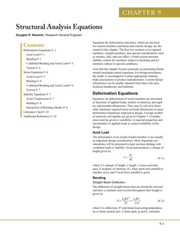
CIVL 7/8117Chapter 4 - Development of Beam Equations - Part 1Beam Stiffness( ) Shear Force(-) Shear ForceBeam StiffnessThe differential equation governing simple linear-elastic beambehavior can be derived as follows. Consider the beamshown below.6/39
CIVL 7/8117Chapter 4 - Development of Beam Equations - Part 1Beam StiffnessThe differential equation governing simple linear-elastic beambehavior can be derived as follows. Consider the beamshown below.w ( x )dx dx 2 Write the equations of equilibrium for the differential element: dx Mright side 0 M M dM Vdx w ( x )dx 2 0 F 0 V (V dV ) w ( x )dx yBeam StiffnessFrom force and moment equilibrium of a differential beamelement, we get: M Fyright side 0 0 Vdx dM 0 wdx dV 0oror V dMdxw dVdxw d dM dx dx 7/39
CIVL 7/8117Chapter 4 - Development of Beam Equations - Part 1Beam StiffnessThe curvature of the beam is related to the moment by: 1 MEIwhere is the radius of the deflected curve, v is thetransverse displacement function in the y direction, E is themodulus of elasticity, and I is the principle moment of inertiaabout y direction, as shown below.Beam StiffnessThe curvature, for small slopes d 2v 2dxTherefore:d 2v M dx 2 EI dvis given as:dxM EId 2vdx 2Substituting the moment expression into the moment-loadequations gives:d 2 d 2v EI w x dx 2 dx 2 For constant values of EI, the above equation reduces to: d 4v EI 4 w x dx 8/39
CIVL 7/8117Chapter 4 - Development of Beam Equations - Part 1Beam StiffnessStep 1 - Select Element TypeWe will consider the linear-elastic beam element shown below.Beam StiffnessStep 2 - Select a Displacement FunctionAssume the transverse displacement function v is:v a1x 3 a2 x 2 a3 x a4The number of coefficients in the displacement function ai isequal to the total number of degrees of freedom associatedwith the element (displacement and rotation at each node).The boundary conditions are:v ( x 0) v1v ( x L) v 2dvdxdvdx 1x 0 2x L9/39
CIVL 7/8117Chapter 4 - Development of Beam Equations - Part 110/39Beam StiffnessStep 2 - Select a Displacement FunctionApplying the boundary conditions and solving for the unknowncoefficients gives:v (0) v1 a4v (L ) v 2 a1L3 a2L2 a3L a4dv (0) 1 a3dxdv (L ) 2 3a1L2 2a2L a3dxSolving these equations for a1, a2, a3, and a4 gives:1 2 v 3 v1 v 2 2 1 2 x 3L L 1 3 2 v1 v 2 2 1 2 x 2 1x v1L L Beam StiffnessStep 2 - Select a Displacement FunctionIn matrix form the above equations are: v [N ] d v1 d 1 v 2 2 where[N ] N1 N2 N3 N4 N1 12 x 3 3 x 2L L3L3N3 1 2 x 3 3 x 2 LL3 N2 1 3x L 2 x 2L2 xL3L3N4 1 3x L x 2L2L3
CIVL 7/8117Chapter 4 - Development of Beam Equations - Part 1Beam StiffnessStep 2 - Select a Displacement FunctionN1, N2, N3, and N4 are called the interpolation functions for abeam 000.0000.00-0.2001.00N40.0000.001.00-0.200Beam StiffnessStep 3 - Define the Strain/Displacementand Stress/Strain RelationshipsThe stress-displacement relationship is: x x, y where u is the axial displacement function.dudxWe can relate the axial displacement to the transversedisplacement by considering the beam element shownbelow:11/39
CIVL 7/8117Chapter 4 - Development of Beam Equations - Part 1Beam StiffnessStep 3 - Define the Strain/Displacementand Stress/Strain Relationshipsu ydvdxBeam StiffnessStep 3 - Define the Strain/Displacementand Stress/Strain RelationshipsOne of the basic assumptions in simple beam theory is thatplanes remain planar after deformation, therefore: x x, y d 2v du y 2 dx dx Moments and shears are related to the transversedisplacement as: d 2v m x EI 2 dx d 3v V x EI 3 dx 12/39
CIVL 7/8117Chapter 4 - Development of Beam Equations - Part 113/39Beam StiffnessStep 4 - Derive the Element Stiffness Matrixand EquationsUse beam theory sign convention for shear force and bendingmoment.M M V V Beam StiffnessStep 4 - Derive the Element Stiffness Matrixand EquationsUsing beam theory sign convention for shear force andbending moment we obtain the following equations:f1y V EIf2 yd 3vdx 3 x 0d 3v V EI 3dxm1 m EI EI 12v1 6L 1 12v 2 6L 2 L3 EI6Lv1 4L2 1 6Lv 2 2L2 23Lx L2d vdx 2d 2vm2 m EI 2dxEI 12v1 6L 1 12v 2 6L 2 L3x 0 x L EI6Lv1 2L2 1 6Lv 2 4L2 23L
CIVL 7/8117Chapter 4 - Development of Beam Equations - Part 1Beam StiffnessStep 4 - Derive the Element Stiffness Matrixand EquationsIn matrix form the above equations are: f1y 12 m 1 EI 6L 3 f2 y L 12 m2 6L6L4L2 6L 12 6L122L2 6L6L v1 2L2 1 6L v 2 4L2 2 f1y v1 m 1 1 k f2 y v 2 m2 2 where the stiffness matrix is: 12 EI 6Lk 3 L 12 6L6L 124L2 6L 6L122L2 6L6L 2L2 6L 4L2 Beam StiffnessStep 4 - Derive the Element Stiffness Matrixand EquationsBeam stiffness based on Timoshenko Beam TheoryThe total deflection of the beam at a point x consists of twoparts, one caused by bending and one by shear force. Theslope of the deflected curve at a point x is:dv x x dx14/39
CIVL 7/8117Chapter 4 - Development of Beam Equations - Part 1Beam StiffnessStep 4 - Derive the Element Stiffness Matrixand EquationsBeam stiffness based on Timoshenko Beam TheoryThe relationship between bending moment and bendingdeformation is:d x M x EIdxBeam StiffnessStep 4 - Derive the Element Stiffness Matrixand EquationsBeam stiffness based on Timoshenko Beam TheoryThe relationship between shear force and shear deformation is:V x ks AG x where ksA is the shear area.15/39
CIVL 7/8117Chapter 4 - Development of Beam Equations - Part 1Beam StiffnessStep 4 - Derive the Element Stiffness Matrixand EquationsBeam stiffness based on Timoshenko Beam TheoryYou can review the details in your book, but by including theeffects of shear deformations into the relationship betweenforces and nodal displacements a modified elementalstiffness can be developed.Beam StiffnessStep 4 - Derive the Element Stiffness Matrixand EquationsBeam stiffness based on Timoshenko Beam Theory 12 EI 6Lk 3L 1 12 6L6L 4 L2 6L 2 L2 12 6L12 6L6L 2 L2 6L 4 L2 12EIks AGL216/39
CIVL 7/8117Chapter 4 - Development of Beam Equations - Part 1Beam StiffnessStep 5 - Assemble the Element Equationsand Introduce Boundary ConditionsConsider a beam modeled by two beam elements (do notinclude shear deformations):Assume the EI to be constant throughout the beam. A force of1,000 lb and moment of 1,000 lb-ft are applied to the midpoint of the beam.Beam StiffnessStep 5 - Assemble the Element Equationsand Introduce Boundary ConditionsThe beam element stiffness matrices are: 1v1k (1) 12 EI 6L 3L 12 6Lvk (2)2 12 EI 6L 3 L 12 6L6L4L2 6L2L2 26L4L2 6L2L2v2 12 6L12 6Lv3 12 6L12 6L 26L 2L2 6L 4L2 36L 2L2 6L 4L2 17/39
CIVL 7/8117Chapter 4 - Development of Beam Equations - Part 1Beam StiffnessStep 5 - Assemble the Element Equationsand Introduce Boundary ConditionsIn this example, the local coordinates coincide with the globalcoordinates of the whole beam (therefore there is notransformation required for this problem).The total stiffness matrix can be assembled as: F1y 126L6L00 v1 12 M 6L 4L22 6L2L00 1 1 F2 y EI 12 6L 12 12 6L 6L 12 6L v 2 M 3 2222 2 L 6L 2L 6L 6L 4L 4L 6L 2L 2 F3 y 0 12 6L012 6L v 3 2 6L 4L2 3 06L2L M3 0Element 1Element 2Beam StiffnessStep 5 - Assemble the Element Equationsand Introduce Boundary ConditionsThe boundary conditions are:v1 1 v 3 0 F1y 6L6L 12 12 M 6L 4L22L2 6L 1 F2 y EI 12 6L 12 12 6L 6L M 3 222 2 L 6L 2L 6L 6L 4L 4L F3 y 00 12 6L 06L2L2 M3 00 v01 0 01 6L v 2 2L2 2 12 6L v03 6L 4L2 3 00 12 6L18/39
CIVL 7/8117Chapter 4 - Development of Beam Equations - Part 1Beam StiffnessStep 5 - Assemble the Element Equationsand Introduce Boundary ConditionsBy applying the boundary conditions the beam equationsreduce to:6L v 2 1,000 lb 24 0 EI 22 1,000 lb ft 3 0 8L 2L 2 L 6L 2L2 4L2 0 3 Beam StiffnessStep 6 - Solve for the Unknown Degrees of FreedomSolving the above equations gives:v2 875L3 375L2in12EI 2 125L2 625Lrad4EI 3 125L2 125LradEIStep 7 - Solve for the Element Strains and Stresses v1 22 d v d N m x EI 2 EI 2 1 dx v 2 dx 2 The second derivative of N is linear; therefore m(x) is linear.19/39
CIVL 7/8117Chapter 4 - Development of Beam Equations - Part 1Beam StiffnessStep 6 - Solve for the Unknown Degrees of FreedomSolving the above equations gives:v2 875L3 375L2in12EI 2 125L2 625Lrad4EI 3 125L2 125LradEIStep 7 - Solve for the Element Strains and Stresses v1 3 d v d 3N 1 V x EI 3 EI 2 dx dx v 2 2 The third derivative of N is a constant; therefore V(x) isconstant.Beam StiffnessStep 7 - Solve for the Element Strains and StressesAssume L 120 in, E 29x106 psi, and I 100 in4: 2 7.758 10 5 radv 2 0.0433 in 3 5.586 10 4 radElement #1: v1 d v d N 1 m x EI 2 EI 2 dx v 2 dx 2 22EI6Lv1 4L2 1 6Lv 2 2L2 2 3,875 lb ftL3EIm2 3 6Lv1 2L2 1 6Lv 2 4L2 2 3,562.5 lb ftLm1 20/39
CIVL 7/8117Chapter 4 - Development of Beam Equations - Part 1Beam StiffnessStep 7 - Solve for the Element Strains and StressesAssume L 120 in, E 29x106 psi, and I 100 in4: 2 7.758 10 5 radv 2 0.0433 in 3 5.586 10 4 radElement #2: v1 d v d N m x EI 2 EI 2 1 dx v 2 dx 2 22EI6Lv 2 4L2 2 6Lv 3 2L2 3 2,562.5 lb ft3LEIm3 3 6Lv 2 2L2 2 6Lv 3 4L2 3 0Lm2 Beam StiffnessStep 7 - Solve for the Element Strains and StressesAssume L 120 in, E 29x106 psi, and I 100 in4: 2 7.758 10 5 radv 2 0.0433 in 3 5.586 10 4 radElement #1: v1 d v d N V x EI 3 EI 2 1 dx dx v 2 2 EIf1y 3 12v1 6L 1 12v 2 6L 2 L3f2 y 3 743.75 lbEI 12v1 6L 1 12v 2 6L 2 743.75 lbL321/39
CIVL 7/8117Chapter 4 - Development of Beam Equations - Part 1Beam StiffnessStep 7 - Solve for the Element Strains and StressesAssume L 120 in, E 29x106 psi, and I 100 in4:v 2 0.0433 in 2 7.758 10 5 rad 3 5.586 10 4 radElement #2: v1 d 3v d 3N V x EI 3 EI 2 1 dx dx v 2 2 EIf2 y 3 12v 2 6L 2 12v 3 6L 3 256.25 lbLf3 y EI 12v 2 6L 2 12v 3 6L 3 256.25 lbL3Beam StiffnessStep 7 - Solve for the Element Strains and Stresses 256.25 lb F 1,000 lb743.75 lb3,562.5 lb ft 3,875 lb ft2,562.5 lb ft M 1,000 lb ft22/39
CIVL 7/8117Chapter 4 - Development of Beam Equations - Part 1Beam StiffnessExample 1 - Beam ProblemConsider the beam shown below. Assume that EI is constantand the length is 2L (no shear deformation).The beam element stiffness matrices are:vk (1)1 12 EI 6L 3 L 12 6L 1v26L4L2 12 6L 6L2L212 6L 26L 2L2 6L 4L2 vk (2)2 12 EI 6L 3 L 12 6L 2v6L 122 6L12 6L4L 6L2L2 336L 2L2 6L 4L2 Beam StiffnessExample 1 - Beam ProblemThe local coordinates coincide with the global coordinates ofthe whole beam (therefore there is no transformation requiredfor this problem).The total stiffness matrix can be assembled as: F1y 6L 12 6L00 v1 12 M 6L 4L2 6L 2L200 1 1 F2 y EI 12 6L 240 12 6L v 2 M 3 2208L 6L 2L2 2 2 L 6L 2L F3 y 00 12 6L 12 6L v 3 06L 2L2 6L 4L2 3 0 M3 Element 1Element 223/39
CIVL 7/8117Chapter 4 - Development of Beam Equations - Part 1Beam StiffnessExample 1 - Beam ProblemThe boundary conditions are:v 2 v 3 3 0 F1y 6L 12 6L00 v1 12 M 6L 4L2 6L 2L200 1 1 F2 y EI 12 6L 24 12 6L v02 0 M 3 208L2 6L 2L2 2 2 L 6L 2L F3 y 00 12 6L 12 6L v03 06L 2L2 6L 4L2 03 M3 0Beam StiffnessBy applying the boundary conditions the beam equationsreduce to:6L 6L v1 P 12 EI 22 0 3 6L 4L 2L 1 0 L 6L 2L2 8L2 2 Solving the above equations gives: 7L 3 v1 2 PL 1 3 4EI 2 1 24/39
CIVL 7/8117Chapter 4 - Development of Beam Equations - Part 1Beam StiffnessExample 1 - Beam ProblemThe positive signs for the rotations indicate that both are in thecounterclockwise direction.The negative sign on the displacement indicates a deformationin the -y direction. F1y 6L 12 6L00 7 L 3 12 M 6L 4L2 6L 2L200 3 1 F2 y P 12 6L 24 12 6L 0 0 M 208L2 6L 2L2 1 2 4L 6L 2L F3 y 0 12 6L 12 6L 0 0 06L 2L2 6L 4L2 0 M3 0Beam StiffnessExample 1 - Beam ProblemThe local nodal forces for element 1:6L 12 6L 7L 3 P f1y 12 22 m1 P 6L 4L 6L 2L 3 0 f2 y 4L 12 6L 12 6L 0 P 22 m2 6L 2L 6L 4L 1 PL The local nodal forces for element 2:6L 12 6L 0 1.5P f2 y 12 m 6L 4L2 6L 2L2 1 PL 2 P f3 y 4L 12 6L 12 6L 0 1.5P 22 m3 6L 2L 6L 4L 0 0.5PL 25/39
CIVL 7/8117Chapter 4 - Development of Beam Equations - Part 1Beam StiffnessExample 1 - Beam ProblemThe free-body diagrams for the each element are shownbelow.Combining the elements gives the forces and moments for theoriginal beam.Beam StiffnessExample 1 - Beam ProblemTherefore, the shear force and bending moment diagrams are:26/39
CIVL 7/8117Chapter 4 - Development of Beam Equations - Part 1Beam StiffnessExample 2 - Beam ProblemConsider the beam shown below. Assume E 30 x 106 psi andI 500 in4 are constant throughout the beam. Use fourelements of equal length to model the beam.The beam element stiffness matrices are:vik( i ) 12 EI 6L 3L 12 6L iv ( i 1) ( i 1)6L4L2 12 6L 6L2L212 6L6L 2L2 6L 4L2 Beam StiffnessExample 2 - Beam ProblemUsing the direct stiffness method, the four beam elementstiffness matrices are superimposed to produce the globalstiffness matrix.Element 1Element 2Element 3Element 427/39
CIVL 7/8117Chapter 4 - Development of Beam Equations - Part 1Beam StiffnessExample 2 - Beam ProblemThe boundary conditions for this problem are:v1 1 v 3 v 5 5 0Beam StiffnessExample 2 - Beam ProblemThe boundary conditions for this problem are:v1 1 v 3 v 5 5 0After applying the boundary conditions the global beamequations reduce to: 24 0 0 8L2EI 6L 2L23L 0 0 000 v 2 10,000 lb 00 2 08L2 6L 2L2 3 v 10,000 lb 0 4 6L 24 202L0 8L2 4 6L2L20028/39
CIVL 7/8117Chapter 4 - Development of Beam Equations - Part 1Beam StiffnessExample 2 - Beam ProblemSubstituting L 120 in, E 30 x 106 psi, and I 500 in4 intothe above equations and solving for the unknowns gives: 2 3 4 0v 2 v 4 0.048 inThe global forces and moments can be determined as:F1y M1 5 kips25 kipsꞏftF2 y 10 kipsF3 y 10 kipsM2 0M3 0F4 y 10 kipsF5 y 5 kipsM4 0M5 25 kipsꞏftBeam StiffnessExample 2 - Beam ProblemThe local nodal forces for element 1: f1y 12 m 1 EI 6L 3 f2 y L 12 6L m2 6L 124L2 6L 6L2L212 6L6L 0 5 kips 2L2 0 25 kꞏft 6L 0.048 5 kips 4L2 0 25 kꞏft The local nodal forces for element 2: f2 y 12 m 2 EI 6L 3 f3 y L 12 6L m3 6L 1224L 6L 6L2L212 6L6L 0.048 5 kips 2L2 0 25 kꞏft 6L 0 5 kips 4L2 0 25 kꞏft 29/39
CIVL 7/8117Chapter 4 - Development of Beam Equations - Part 1Beam StiffnessExample 2 - Beam ProblemThe local nodal forces for element 3: f3 y 12 m 3 EI 6L 3 f4 y L 12 6L m4 6L 1224L 6L 6L2L212 6L6L 0 5 kips 2L2 0 25 kꞏft 6L 0.048 5 kips 4L2 0 25 kꞏft The local nodal forces for element 4: f4 y 12 m 4 EI 6L 3 f5 y L 12 6L m5 6L 124L2 6L 6L2L212 6L6L 0.048 5 kips 2L2 0 25 kꞏft 6L 0 5 kips 4L2 0 25 kꞏft Beam StiffnessExample 2 - Beam ProblemNote: Due to symmetry about the vertical plane at node 3, wecould have worked just half the beam, as shown below.Line of symmetry30/39
CIVL 7/8117Chapter 4 - Development of Beam Equations - Part 1Beam StiffnessExample 3 - Beam ProblemConsider the beam shown below. Assume E 210 GPa andI 2 x 10⁻⁴ m4 are constant throughout the beam and thespring constant k 200 kN/m. Use two beam elements ofequal length and one spring element to model the structure.Beam StiffnessExample 3 - Beam ProblemThe beam element stiffness matrices are: 1v1k (1) 12 EI 6L 3 L 12 6Lv26L 124L2 6L2L2 6L12 6L 2v26L 2L2 6L 4L2 k (2) 12 EI 6L 3 L 12 6L 26L 124L2 6L2L2 6LThe spring element stiffness matrix is:v3k(3) k kv3v4 k k k(3) 3v3v4 k 0 k 0 0 0 k 0 k 12 6L 36L 2L2 6L 4L2 31/39
CIVL 7/8117Chapter 4 - Development of Beam Equations - Part 132/39Beam StiffnessExample 3 - Beam ProblemUsing the direct stiffness method and superposition gives theglobal beam equations.Element 1Element 2 F1y 6L 12 6L000 v1 12 M 6L 4L2 6L 2L2000 1 1 F2 y 12 6L 2406L0 v 2 12 EI 208L22L20 2 6L M2 3 6L 2LL F 00 12 6L 12 k ' 6L k ' v 3 3y 220062640 LLLL M3 3 F 0000 k 'k ' v 4 0 4y k' kL3EIElement 3Beam StiffnessExample 3 - Beam ProblemThe boundary conditions for this problem are: v1 1 v 2 v 4 0 F1y 6L 12 6L000 v01 12 M 6L 4L2 6L 2L2000 01 1 F2 y 12 6L 24 1206L0 v02 EI 2 6L08L22L20 2 M2 3 6L 2LL F 0 12 6L 12 k ' 6L k ' v 3 0 3y 22LLLL 0062640 M3 3 F v04 kk 0000'0' 4y k' kL3EI
CIVL 7/8117Chapter 4 - Development of Beam Equations - Part 1Beam StiffnessExample 3 - Beam ProblemAfter applying the boundary conditions the global beamequations reduce to: 8L2 6L2L2 2 0 M2 EI F3 y 3 6L 12 k ' 6L v 3 P M L 2L2 6L4L2 3 0 3 Solving the aboveequations gives: 3PL2 1 EI 12 7k ' 2 31 7PL v 3 EI 12 7k ' 3 9PL2 1 EI 12 7k ' k' kL3EIBeam StiffnessExample 3 - Beam ProblemSubstituting L 3 m, E 210 GPa, I 2 x 10⁻⁴ m4, andk 200 kN/m in the above equations gives:v 3 0.0174 m 2 0.00249 rad 3 0.00747 radSubstituting the solution back into the global equations gives: F1y 6L 12 6L000 0 12 M 6L 4L2 6L 2L2 00001 F2 y 12 6L 24 1206L0 0 EI 222M 6L08L2L0 0.00249 rad 2 3 6L 2LL F 0 12 6L 12 k ' 6L k ' 0.0174 m 0 3y 6L06L 2L24L20 0.00747 rad M3 0 F 0k ' k '00000 4y 33/39
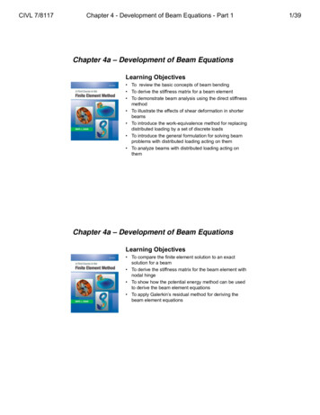
CIVL 7/8117Chapter 4 - Development of Beam Equations - Part 1Beam StiffnessExample 3 - Beam ProblemSubstituting L 3 m, E 210 GPa, I 2 x 10⁻⁴ m4, andk 200 kN/m in the above equations gives:v 3 0.0174 m 2 0.00249 rad 3 0.00747 radSubstituting the solution back into the global equations gives: F1y 69.9 kN M 1 69.7 kN m F2 y 116.4 kN 0 M2 F 50 kN 3y 0 M3 F 3.5 kN 4y Beam StiffnessExample 3 - Beam ProblemThe variation of shear force and bending moment is: 69.9 kN46.5 kN69.7 kNm 139.5 kNm34/39
CIVL 7/8117Chapter 4 - Development of Beam Equations - Part 1Beam StiffnessDistributed LoadingsBeam members can support distributed loading as well asconcentrated nodal loading.Therefore, we must be able to account for distributed loading.Consider the fixed-fixed beam subjected to a uniformlydistributed loading w shown the figure below.The reactions, determined from structural analysis theory, arecalled fixed-end reactions.Beam StiffnessDistributed LoadingsIn general, fixed-end reactions are those reactions at the endsof an element if the ends of the element are assumed to befixed (displacements and rotations are zero).Therefore, guided by the results from structural analysis for thecase of a uniformly distributed load, we replace the load byconcentrated nodal forces and moments tending to have thesame effect on the beam as the actual distributed load.35/39
CIVL 7/8117Chapter 4 - Development of Beam Equations - Part 1Beam StiffnessDistributed LoadingsThe figures below illustrates the idea of equivalent nodal loadsfor a general beam. We can replace the effects of a uniformload by a set of nodal forces and moments.Beam StiffnessWork Equivalence MethodThis method is based on the concept that the work done bythe distributed load is equal to the work done by the discretenodal loads. The work done by the distributed load is:LWdistributed w x v x dx0where v(x) is the transverse displacement. The work done bythe discrete nodal forces is:Wnodes m1 1 m2 2 f1y v1 f2 y v 2The nodal forces can be determined by settingWdistributed Wnodes for arbitrary displacements and rotations.36/39
CIVL 7/8117Chapter 4 - Development of Beam Equations - Part 1Beam StiffnessExample 4 - Load ReplacementConsider the beam, shown below, and determine theequivalent nodal forces for the given distributed load.Using the work equivalence method or:L w x v x dx m 1 1Wdistributed Wnodes m2 2 f1y v1 f2 y v 20Beam StiffnessExample 4 - Load ReplacementEvaluating the left-hand-side of the above expression with:w x w1 2 v ( x ) 3 v1 v 2 2 1 2 x 3L L 31 2 v1 v 2 2 1 2 x 2 1x v1L L gives:L w v x dx 0 LwL2w v1 v 2 1 2 Lw v 2 v1 24L2wL2w 2 1 2 1 wLv13237/39
CIVL 7/8117Chapter 4 - Development of Beam Equations - Part 1Beam StiffnessExample 4 - Load ReplacementUsing a set of arbitrary nodal displacements, such as:v1 v 2 2 0 1 1The resulting nodal equivalent force or moment is:Lm1 1 m2 2 f1y v1 f2 y v 2 w x v x dx0 wL2 2 2L2 wL2m1 Lw w 32 12 4Beam StiffnessExample 4 - Load ReplacementUsing a set of arbitrary nodal displacements, such as:v1 v 2 1 0 2 1The resulting nodal equivalent force or moment is:Lm1 1 m2 2 f1y v1 f2 y v 2 w x v x dx0 wL2 wL2 wL2m2 43 1238/39
CIVL 7/8117Chapter 4 - Development of Beam Equations - Part 1Beam StiffnessExample 4 - Load ReplacementSetting the nodal rotations equal zero except for the nodaldisplacements gives:LWLwf1y Lw Lw 22f2 y LWLw Lw 22Summarizing, the equivalent nodal forces and moments are:End of Chapter 4a39/39
Step 3 - Define the Strain/Displacement and Stress/Strain Relationships dv uy dx Beam Stiffness Step 3 - Define the Strain/Displacement and Stress/Strain Relationships One of the basic assumptions in simple beam theory is that planes remain planar after deformation, therefore: Moments and sh