Transcription
Queues with Time-Dependent Arrival Rates I:The Transition through SaturationAuthor(s): G. F. NewellSource: Journal of Applied Probability, Vol. 5, No. 2 (Aug., 1968), pp. 436-451Published by: Applied Probability TrustStable URL: http://www.jstor.org/stable/3212264Accessed: 03-08-2016 19:33 UTCYour use of the JSTOR archive indicates your acceptance of the Terms & Conditions of Use, available athttp://about.jstor.org/termsJSTOR is a not-for-profit service that helps scholars, researchers, and students discover, use, and build upon a wide range of content in a trusteddigital archive. We use information technology and tools to increase productivity and facilitate new forms of scholarship. For more information aboutJSTOR, please contact support@jstor.org.Applied Probability Trust is collaborating with JSTOR to digitize, preserve and extend access to Journalof Applied ProbabilityThis content downloaded from 128.59.222.107 on Wed, 03 Aug 2016 19:33:17 UTCAll use subject to http://about.jstor.org/terms
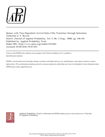
J. Appl. Prob. 5, 436-451 (1968)Printed in IsraelQUEUES WITH TIME-DEPENDENT ARRIVAL RATESI-THE TRANSITION THROUGH SATURATIONG. F. NEWELL, Institute of Transportation and Traffic Engineering,University of California, BerkeleyAbstractSuppose that the arrival rate A(t) of customers to a service facility increaseswith time at a nearly constant rate, dA(t)/dt a, so as to pass through thesaturation condition, ,A(t) t service capacity, at some time which welabel as t 0. The stochastic properties of the queue are investigated herethrough use of the diffusion approximation (Fokker-Planck equation). It isshown that there is a characteristic time T proportional to a-2/3 such that ift 0, jt T, then the queue distribution stays close to the prevailing equilibrium distribution associated with the A(t) and #,, evaluated at time t. Forit O(T), however, the mean queue length is much less than the equilibriummean, and is measured in units of some characteristic length L which is propor-tional to a-1/3. For t 0, It 1 T, the queue is approximately normallydistributed with a mean of the order L larger than that predicted by deterministic queueing models. Numerical estimates are given for the mean andvariance of the distribution for all t. The queue distributions are also evaluatedin non-dimensional units.1. IntroductionIt is quite common in practical queueing situations that customers arrive at aservice facility with an arrival rate A(t) which is significantly time dependent.Frequently the arrival rate gradually increases as a "rush hour" approachesuntil 2(t) actually exceeds the service capacity of the server. Eventually the arrivalrate subsides again and the queue which builds up during the rush hour is workedoff.Situations of this type are customarily analyzed only by means of deterministicqueueing models [1-3]. We draw a graph of the expected cumulative numberof arrivals to time t, E{A(t)}, versus t as in Figure 1 and treat this as if it werethe actual number of arrivals. As long as the slope of this curve, the arrival rate2(t), stays less than the service rate p, we approximate the queue to be zero andsay that the (expected) cumulative number of departures to time t, E{D(t)}, isequal to E{A(t)}. But as soon as A(t) exceeds p, we draw the expected departurecurve with a slope p (also treated as if it were the actual departure curve) untilE{D(t)} is again equal to E{A(t)}, after the rush hour is over. Thus the (possiblyReceived'21 October 1967.436This content downloaded from 128.59.222.107 on Wed, 03 Aug 2016 19:33:17 UTCAll use subject to http://about.jstor.org/terms
Queues with time-dependent arrival rates. I: The transition through saturation 437/3iSI/S Arrivals // I DepartureE Slope X(f) / Slope 0 t, Time -tFigure 1stochastic) queueing phenomena are represented as if customers were a fluidwhich is poured into a reservoir having a capacity flow rate p. The expectedqueue length at any time t (fluid in the reservoir) is E{A(t) - D(t)}, the verticaldistance between the two curves.To analyze some of the consequences of statistical fluctuations in the arrivaland service rates for a situation like this, we should interpret A(t) and D(t) asrandom functions of time, the expectations of which have time derivatives A(t)and respectively; the latter, however, only when the actual queue is nonzero.If we define t 0 as the time when A(t) y, we would not anticipate a vanishingexpected queue even for t 0, certainly not for t10O. It is also clear that the expectedqueue length at t 0 must depend upon the rate at which the arrival rate buildsup to the value u at t 0. If at one extreme, the arrival rate builds up very sud-denly (dA(t)/dt oo) from a value A(t) 0 for t 0 to a value of y at t 0, thequeue will be zero as t t0. On the other hand, if the arrival rate increases verygradually (dA(t)/dt - 0) the queue length distribution will try to adjust tothe equilibrium queue distribution at the prevailing traffic intensity, )(t)/p. Theequilibrium mean queue length becomes infinite, however, as the traffic intensityapproaches 1 at t 0. For any finite rate of approach to the critical arrival rate,the expected queue length at t 0 must have some finite value between thesetwo extremes of 0 and oo.Deterministic queueing approximations always tend to underestimate theexpected queue length. In particular for t 0, the expected departure curvewould have slope exactly y if the departure process could proceed independentlyof the queue length, even if the queue length wanted to become negative. Forthe real queueing process, however, the service might be interrupted if the queueThis content downloaded from 128.59.222.107 on Wed, 03 Aug 2016 19:33:17 UTCAll use subject to http://about.jstor.org/terms
438G.F.NEWELLvanishes. The actual average service rate can never be larger than Yu. Duringthe time when the deterministic model predicts a nonzero queue, the differencebetween the actual expected queue length and the deterministic estimate istherefore nondecreasing in time, and is at least as large for t 0 as the actualexpected queue at t 0, i.e., somewhere between 0 and oo. Even some crudeestimates of the order of magnitude of this difference would obviously be ofsome practical value.2. Diffusion approximationThere is little likelihood that anyone will find a queueing model with a timedependent arrival rate of the above type which is sufficiently simple as to yieldexact solutions in any usable form. We shall, therefore, immediately attack thisproblem by approximate methods.The "second order" approximation, after the deterministic model, is the"diffusion" model [4], [5]. This is also based upon the postulate that the queuesare almost always long enough so that one can disregard the discrete natureof customers. In fact, the queues are so long that one can find a scale of time zsufficiently short that during a time z the fractional change in the queue duringtime z is small (most of the time), yet z is sufficiently large that during time zthere are many arrivals and departures from the queue. Furthermore, the numberof arrivals and departures during z are approximately normally distributed.The corresponding postulates for the deterministic approximation would implythat r was long enough that one could apply a law of large numbers instead ofa central limit theorem, thus neglecting fluctuations completely. These approximations obviously are not accurate when the traffic intensity is well below 1for t 0, but the queue is too small to be of any interest then anyway.These postulates lead to a diffusion equation (Fokker-Planck equation) forthe queue length. If we assume that behaviors of the arrival and service do notdepend explicitly on the queue length (except when the queue length is zero),we letX(t) queue length at time t,and(1) F(x, t) P(X(t) x}be the distribution function for the queue length at time t, then F(x, t) satisfies(approximately) an equation of the type, [6], (2) F(x, t) ataOF(x,ax t) b(t)2 02F(x,ax2 t)This equation differs from the more familiar differential equation for a homogeneous process only in that the coefficients a(t) and b(t) depend upon t here.This content downloaded from 128.59.222.107 on Wed, 03 Aug 2016 19:33:17 UTCAll use subject to http://about.jstor.org/terms
Queues with time-dependent arrival rates. I: The transition through saturation 439In terms of the arrival and departure processes, the coefficients a(t) and b(t)are given by(3) a(t) z-'1E{D(t T) - D(t) - A(t z) A(t)},b(t) z-1Var {D(t z) - D(t) - A(t z) A(t)},i.e., they are respectively the rate of change in the expected queue length andrate of change of the variance of the queue length.It is implied in (3) that there exists a certain range of r over which the righthand sides of (3) are essentially independent of z. This z is small compared withtimes over which the a(t) and b(t) change significantly, so in this sense a(t) andb(t) are instantaneous rates on the time scale of t in (2). However, z is largeenough that many customers arrive or depart during z, so as to give the asymptoticnormal approximation and a variance approximately proportional to z in (3).(The deterministic approximation corresponds to neglect of the second derivativeterm in (2)).In terms of the 1(t) and i(4) a(t) p - A(t).For the most common types of stochastic arrival and departure processes, thevariances and means of cumulative counts for arrivals or departures are comparable. For a Poisson process they are exactly equal. It is convenient then towrite(5) b(t) I,;(t) I,for some suitable coefficients I, and I, which we would expect to be comparablewith 1 and essentially independent of the 2(t) or p.Equation (2) is to be solved subject to the boundary condition that(6a) F(x,t)- 1 for x-* co,(6b) F(x,t)- O for x- 0,and(6c) F(x,t)- l for x 0, t- -oo.Condition (6a) is the necessary condition for a proper random variable. Condition(6b) implies that X(t) O0. Actually one could admit a slight discontinuity inF(x, t) at x 0, but to justify the approximations used here, the queue shouldalmost always be large and have very small probability of being exactly zero.Condition (6c) implies that at some time in the distant past when the traffic intensitywas low, the queue length was negligibly small.It is still quite difficult to solve even these approximate equations (2) and (6),This content downloaded from 128.59.222.107 on Wed, 03 Aug 2016 19:33:17 UTCAll use subject to http://about.jstor.org/terms
440G.F.NEWELLbut we can use these equations along with some logical interpretations of queue-ing phenomena to gain further understanding of what is taking place.3. Undersaturated conditionsConsider first the queue behavior for t 0, when a(t) 0. Let us supposethat there is a period of time during which a(t) and b(t) are nearly constant withvalues ao and bo, respectively. The queue distribution will, given sufficient time,approach an equilibrium distribution obtained by setting OF/Ot 0 in (2), namely(7) Fo(x) 1 - exp[-2aox/bo].This is the continuum exponential approximation to the geometric discretedistribution and has a meanbo IPo I0I2o0(8) E{X0 -oIP2ao- 2,uo[1- 0o/o]It is, of course, a formula of this type that tells us that for 0/p0o -- 1, the equi-librium queue length becomes infinite.Equally important here, however, is the rate of approach to the equilibrium.Detailed properties of the transient behavior have been considered by Gaver [8].It suffices here to notice that if we choose new units of time and queue length(9) t' t/To, x' x/Lo,then (2) becomesOF Toao OF Tobo 02F(10) at' -Lo ax' 2L? Ox'2If, in particular, we choose To and Lo so thatToao - 1 and Tob 1,i.e.,Lo Lo(11) Lo bo and aoToaothen the coefficients in (10) become 1 and 1/2.If in this nondimensional form of the diffusion equation we take as an initialstate any queue length of order x' 1, or any nonequilibrium distribution ofqueue lengths over a range x' of order 1, this distribution will relax to the equilibrium distribution within a time t' of order 1. This must be so since there areno parameters in the equation other than constants of order 1. In terms of theoriginal units, we see that Lo is comparable with (actually two times) the averageThis content downloaded from 128.59.222.107 on Wed, 03 Aug 2016 19:33:17 UTCAll use subject to http://about.jstor.org/terms
Queues with time-dependent arrival rates. I: The transition through saturation 441equilibrium queue length, as would be expected. The unit of time, however, isproportional to ao 2 . As the traffic intensity approaches 1, ao - 0, the relaxationtime becomes large like ao2 whereas the queue length becomes large only as-1a0Let us now return to the question of what happens if a(t) and b(t) (particularlya(t)) are time dependent, slowly varying (in some sense) functions of time witha(t) - 0 as t - 0. If at some time to we have coefficientsa(to) ao, b(to) bo,and we change units of time (relative to to as a new origin) and queue lengtht to Tot', x x'Lo,then (2) becomesaF a(to Tot') aF b(to Tot') a2Fat' ao 0 x' 2bo x'92If the coefficients in this equation, considered as functions of t', are nearlyconstant over a t' range of order 1, for example if1 da(to Tot') I TO da(t)ao dt' ao dtand?11 db(to Tot') I TO db(t)Ibo dt' bo dt 'then any deviations from an equilibrium distribution will have time to relaxbefore the equilibrium distribution can change very much.We thus conclude that for any range of time where(12) b(t) da(t) 1, 1 db(t) I and a(t) O,a3(t) dt Ila2(t) dtthe queue length distribution will at all times stay close to the prevailing equilibrium distribution, i.e.,(13) F(x, t) 1I - exp [- 2a(t)x/b(t)].In practical applications there is no reason why as t - 0, A(t) should increasein any way other than linearly. It is reasonable to postulate, therefore, that insome neighborhood of t 0(14) a(t) - (t) - atfor some constant t, andb(t) I M(t) I,g z (IA I,)M IRclt.This content downloaded from 128.59.222.107 on Wed, 03 Aug 2016 19:33:17 UTCAll use subject to http://about.jstor.org/terms
442G.F.NEWELLIn this case conditions (12) for the validity of (13) are that(5at ?(I l)a)1 Ot t Ift)1/2(15)22and t 0.The quantity a/#2 in (15) is a dimensionless parameter which can be interpretedas the fractional change in arrival rate during an interarrival time. The diffusionequation is meaningless unless this is very small compared with 1. In all practicalcases or any meaningful application of the approximations the second inequalityabove is implied by the first, i.e., the time dependence of the b(t) is of little con-sequence near t 0.The implication of the above conditions are that as t approaches zero and theequilibrium average queue length becomes large, there comes a time when thequeue can no longer grow fast enough to keep up with the equilibrium distribution. There is a characteristic time T such that as t/T becomes of order 1, (15)breaks down. We will further confirm later that this time T given byaT .(1l I2) 1}2(16a)T -(I II)"3 (t22/3is the "natural" unit of time for describing the queue behavior near t 0. Fort - T, we also expect the queue length to be of the order of magnitude(16b) L - T) a( (I T),)2/3awhich will become the natural unit of queue length near t 0.The most interesting feature of these parameters, T and L, are their dependenceupon a, the rate of increase of the arrival rate at t 0. Tis proportional to a- 2/3and L is proportional to a-1/3. The latter is at least consistent with our earlierprediction that if a d2(t)fdt were infinite, the queue length would be zero att 0; but if a were zero, the mean queue length would be infinite. Why the queuelength should involve the (- 1/3) power of a is certainly less obvious.4. Oversaturated conditionEquation (2) was derived, in essence, from a postulate that queue changes aregenerated from the addition of independent normally distributed random variables,namely arrivals and departures during periods of time of the order of z. Themotivation for the introduction of a differential equation to describe this wasto give a convenient representation of the boundary condition that X(t) 0This content downloaded from 128.59.222.107 on Wed, 03 Aug 2016 19:33:17 UTCAll use subject to http://about.jstor.org/terms
Queues with time-dependent arrival rates. I. The transition through saturation 443for all t. If it were not for this condition prohibiting negative queue lengths,we could very easily have accumulated sums of normal random variables andfound the distribution of X(t) directly.For t 0, the average queue length is certain to increase rapidly with time,and as this happens it also becomes less likely that a fluctuation can cause thequeue to vanish. For a range of t values between some as yet unspecified time tountil the end of the rush hour (as estimated say by the time at which the queuevanishes according to the deterministic model), there should be a negligibleprobability that the queue will vanish at any time. The boundary conditionX(t) ? 0 will not be violated anyway and is redundant.If at time to, we have a queue length xo, then the queue length at time t towill have a conditional distribution F(x, tl xo, to) given bydF(x, t xo, to) 1 [-( - x- m(t, to))2(17) expdx (2rn)/2a(t,to) [ 2a2(t, to)jwhere(18) m(t, to) - a(u)du,t(19) a2(t, to) b(u)du,i.e., it must be normal with the cumulative mean and variances implied by (3).One can readily check that (17) is indeed a solution of (2) for any xo, to.,It also follows that X(t) can be written as the sum of X(to) and a randomvariable X(t Ito) with distribution F(x, t 0, to),. For sufficiently large t, X(t)will also be approximately normal withE{X(t)} -j A - a(u)du,(20)Var {X(t)} B b(u)du,for some suitable numbers A and B which are independent of t. We would alsoexpect thatA-E {X(O)}, B Var {X(0)},since the presence of the reflecting barrier at X(t) 0 for t 0 is expected toincrease the mean and decrease the variance as compared with a free diffusionfrom the queue X(0) at time 0.If the arrival rate increases linearly with time as in (14), thenThis content downloaded from 128.59.222.107 on Wed, 03 Aug 2016 19:33:17 UTCAll use subject to http://about.jstor.org/terms
444G.F.NEWELL(21) a'(t, 0) f b(u)du (I I,)pt,and(22) m(t, 0) - a(u)du t2/2.The a(t,O) has the interpretation of being the spread of the distribution fromdiffusion. It increases as V/t whereas the mean increases as t2. For sufficientlysmall t, the first dominates, but for larger t the latter dominates. The spreadand the mean are comparable when(I, I,)1pt 0 2t4,or(Ia I U)1/3 2)2/3i.e., this occurs when t is of order T, at which time both a(t, 0) and m(t, 0)are of order L. This must also be the order of magnitude of the time to in (17)because once the mean of the queue length begins to dominate the standarddeviation it becomes very unlikely for the queue to vanish. The time T is thusthe order of the time when the queue distribution starts to approach a normaldistribution and drift away from the boundary at x 0.5. Transition behaviorIf over a range of time It O(T), the arrival rate can be approximated by alinear function of t as in (14), we can estimate the queue distribution for t 0and t I O(T) from (13). Also, if we know the queue distribution at some timeto comparable with T, we can estimate the queue distribution for any t tofrom (17), at least until the arrival rate comes down and the queue gets closeto zero again. To find the distribution at time to, however, we must analyzethe queue behavior over the transition region ItI O(T).Over this range of t, we can approximate (2) by(23) OaF aF b(O) 02Fat ax 2 Dax2If we change units of time and length through(24) t* tiT and x* x/L,this equation reduces to the nondimensional form(25) F - aF 1 a2F(25) -ax* 2 ax*,which is still subject to the boundary conditions (6).This content downloaded from 128.59.222.107 on Wed, 03 Aug 2016 19:33:17 UTCAll use subject to http://about.jstor.org/terms
Queues with time-dependent arrival rates. I: The transition through saturation 445Since (25) contains no parameters other than constants of order 1, we wouldexpect all features of the solution to be measured on a scale of order 1 in x*and t*. This further confirms that the queue lengths in the original units mustbe of order L over the range t O(T).From our previous analysis we expect the solution of (25) to behave asymptotically like(26) F(x,t) 1 - exp[ 2t*x*] for t* 0, It*I 1,but for t* 0, t* 1 to be approximately a normal distribution with meant*2/2 0(1) and variance t* 0(1).There does not seem to be any simple analytic solution of (25), but since theequation contains no variable parameters we need determine only one dimensionless solution which then, by appropriate change of units, can be mapped into asolution for any parameters T, L, etc. Or conversely, if we determine by simulation or any other means, the evolution of any distribution which satisfies anequation like (23), we can map it into a solution of (25) or of any other queueingproblem of type (23).6. Numerical solutionThe usual method to integrate numerically an equation like (23) or (25) isto replace it by a finite difference equation. This method, however, can also bedescribed in terms of a hypothetical queueing process in discrete time, or, inthe more common terminology, of a random walk on a lattice with a reflectingbarrier.Suppose we have a sequence of integer valued random variables Xj,j ?.-, -2, -1, 0, 1, 2, ., which represents the queue at time j or theposition of a random walk at time j. LetXXji 1 with probability pjXj 1 Imax (X - 1,0) with probability 1 - pj.i.e., the Xi describe a random walk which at each stage moves up one step ordown one step (if Xj # 0). This differs from the usual random walk with reflecting barrier in that the pj depend upon j. In particular, we will take(27) pj (1 aj)/2, (1 - p) (1 - aj)/2.,for some constant a.The distribution functions for the Xj,F(k) P{X, k)evaluated only at the integer steps, satisfy the finite difference equationsThis content downloaded from 128.59.222.107 on Wed, 03 Aug 2016 19:33:17 UTCAll use subject to http://about.jstor.org/terms
446G.F.NEWELL(28) Fj I(k) pjF,(k1) (1 - pj)Fj(k 1) k - 1,Fj 1(0) (1 --pi)Fj(l).For pj as in (27), and acj 1, Equation (28) is the discrete analogue of thedifferential equation( aFj(k)a2Fj(k)(28a) - aF,(k)18j- akcj2 1ak2Solutions of (27), (28) were evaluated numerically by a computer for severalvalues of a; a 10-1, 2 x 10⁻², and 2 x 10⁻³. This serves two purposes. Firstsince (27), (28) can be interpreted as describing the actual evolution of the distribution functions of a real queue, the behavior of this solution as a function of a,as a decreases, gives an indication of the rate of convergence of the exact solutionto a limit solution, thus an indication of the range of validity of the argumentsdescribed in the previous sections. Secondly, it gives an estimate of the limitsolution which should satisfy (28a), and which, by suitable change in scale, canbe mapped into a solution of (25).If, in (28), we were to freeze the p, at a constant value p, for all j n, thesolution of (28) would converge to the equilibrium solution(29) F,,0(k) 1 - [pn(1 - p,)]k I 1 - [(1 an)/(l - an)]' 'provided n 0. For Inl T 1/a2/3, the solution of (28) at time j n 1should already be close to the equilibrium solution (29) for time n. To obtain anumerical solution of (28), we therefore started from an initial distribution atsome j 0 and moderately large value of I j IT, taking as the initial distribution,the distribution Fj - ,0(k). Values of the Fj 1(k) were then evaluated iterativelyfrom (28) until j reached some positive value of order T and Fj(O) becamenegligible, indicating that the reflecting barrier was no longer of any importance.The pi in (28) are defined as the transition probabilities from stage j to j 1and we have chosen the pj in (27) so that Po 1/2. In order to compare thecalculations for different a, it seemed appropriate to identify a time t - 1/2with the stage j 0 so that Po 1/2 was identified with a transition from time- 1/2 to 1/2. The time t was then rescaled tot* tT ta2/3 (j - 1/2)a2/3,and k was rescaled to* kiL ka1/3Some of the results of the numerical calculations are shown in Figures 2, 3,and 4. Figure 2 shows the evolution of the mean queue length, Figure 3 thevariance, and Figure 4 the distribution functions.This content downloaded from 128.59.222.107 on Wed, 03 Aug 2016 19:33:17 UTCAll use subject to http://about.jstor.org/terms
Queues with time-dependent arrival rates. 1: The transition through saturation 447I13--I o2 -IIII2a 2xl- - ------0.95- a2 2x Queue- 2/a 2xiO,-202Time / 7"Figure 2In Figure 2, the solid line curves shows the mean queue length in units of Lversus t* for a 10-1, 2 x 10⁻², and 2 x 10⁻³. For o 10-1, pj varies allthe way from 0 to 1 while t* ranges from about -2 to 2. The mean queuein original integer units at time 0 is about 1. Despite the fact that the assumptionsof the previous sections (queues large compared with 1, a nearly constant varianceper step over t* 0(1), etc.) are not true for a 10-1, the curve for a 10-1is surprisingly close to those for a 2 x 10⁻² and 2 x 10⁻³.Also shown in Figure 2 is the curve 1/(2t*) which is the mean equilibriumqueue length corresponding to (7) or (26) with b(t) 1 (independent of t) andx(t) xt. The solid curves should, for - 0, be asymptotic to (1/2t*) fort* - - oo. The discrepancy between the solid curves and 1/(2t*) for t* -2is not so much an indication that the queue distribution differs appreciably fromits equilibrium distribution; rather it is a reflection of the fact that for a 0 theeffective b(t) is not sufficiently constant over -2 t* 2. The differencebetween the actual mean and the mean of the correct equilibrium distributionfor oa 0 given by (29) is so small even for t* -1.5 as to hardly show on agraph to the scale of Figure 2.Figure 2, also shows for t 0 the curve t*2/2 which is the queue length as givenby the deterministic queueing theory. The broken line labeled "Queue -t*2/2"is the difference between the queue length for xt 2 x 10⁻³ and the curve t*2/2.This content downloaded from 128.59.222.107 on Wed, 03 Aug 2016 19:33:17 UTCAll use subject to http://about.jstor.org/terms
448G.F.NEWELL3II 1I a,20 6 9a 10-2-02VIISMean ' C000.4--oo0I,-?x'tFigure 4This difference rapidly approaches a constant value of about 0.95 as t* increases.Even for a 10-1 the difference between the actual mean and t*2/2 is about0.76.We thus conclude that the constant A in (20) is(30)A(0.95)L,This content downloaded from 128.59.222.107 on Wed, 03 Aug 2016 19:33:17 UTCAll use subject to http://about.jstor.org/terms
Queues with time-dependent arrival rates. I: The transition through saturation 449and(31) E{X(0)} (0.65)L.Figure 3 shows similar curves for the variances of the queue length (in units of13) versus t*; also the curve 1/(2t*)2 for the variance of the equilibrium distribution with a - 0, and the curve t* for the variance of a diffusion without re-flection from x 0, t 0 with b(t) 1. For the discrete model, the varianceper step is 4p(1 - pj), and for xc 10-1, -2 t* 2, this variance runs from0 to 1 and back to 0. The effect of this shows very clearly in the shape of thecurve for a 10-' near t* 2. It also shows to a lesser extent in the curvefor a 2 x 10⁻²which has a shorter range for pj. The curve for a 2 x 10⁻³does have a nearly constant pj over this range of t* and shows an approach toslope 1 as t* increases.Our main concern is with the behavior of the curves where b(t) is nearly constant.At t* 0, the three curves give very similar values, the curve for a 2 x 10⁻³giving a variance of about 0.32. The dependence upon a seems to show the consequences of two opposing effects. As a decreases, the variance per step increasesfor each fixed t* toward the value 1. This tends to increase the variance of thequeue length also as a - 0. But as a decreases, so also do the time intervalsbetween steps on the t* scale of time. This diffusion therefore feels the reflectingbarrier more often. Reflections off the barrier tend to decrease the variance ofthe queue length. (These two effects both tend to increase the mean queue lengthas a decreases.) One consequence of this competition is that the curves of Figure 3do not approach a limit monotonically as a decreases.Finally, the most important conclusion from Figure 3 is that the varianceof the queue length for small a and large t* is approaching a line of slope 1, whichis about 0.3 below that of a free diffusion from x 0, t* 0. Thus the constantB in (20) is(32) B -(0.3)L2,which is indeed less than Var {X(0)},(33) Var {X(0)} (0.32)L2.The reflecting barrier which for t* 0 could be considered to have caused thequeue to exist at t* 0, will for t* 0 not only wipe out the variance of thequeue which existed at t* 0 but will, in addition, wipe out part of the variancewhich the arrival and departure processes are trying to generate for t 0.Figure 4 shows the distribution functions for the queue length at various valuesof t* with a 2 x 10-. Although these distribution functions are, strictlyspeaking, step functions, they have been smoothed to suggest the shape of thedistribution for cc - 0. The scale of queue length is shown in both the originalThis content downloaded from 128.59.222.107 on Wed, 03 Aug 2016 19:33:17 UTCAll use subject to http://about.jstor.org/terms
450G.F.NEWELLinteger units and the rescaled units x*. The curves are labeled with both therescaled time t* and the values of pj. As t* increases from t* - 1.28 to
queue length at t 0 must depend upon the rate at which the arrival rate builds up to the value u at t 0. If at one extreme, the arrival rate builds up very sud-denly (dA(t)/dt oo) from a value A(t) 0 for t 0 to a value of y at t 0, the queue will be zero as t t0. On the other