Transcription
4CENTRAL FORCE PROBLEMSIntroduction. This is where it all began. Newton’s Mathematical Principles ofNatural Philosophy ( ) was written and published at the insistance of youngEnmund Halley ( – ) so that the world at large might become acquaintedwith the general theory of motion that had permitted Newton to assure Halley(on occasion of the comet of ) that comets trace elliptical orbits (andthat in permitted Halley to identify that comet—now known as “Halley’scomet”—with the comets of and , and to predict its return in ). Itwas with a remarkably detailed but radically innovative account of the quantumtheory of hydrogen that Schrödinger signaled his invention of wave mechanics,a comprehensive quantum theory of motion-in-general. In both instances,description of the general theory was preceded by demonstration of the successof its application to the problem of two bodies in central interaction.1We will be concerned mainly with various aspects of the dynamical problemposed when two bodies interact via central conservative forces. But I would liketo preface our work with some remarks intended to place that problem in itslarger context.We often yield, as classical physicists, to an unexamined predisposition tosuppose that all interactions are necessarily 2-body interactions. To describe asystem of interacting particles we find it natural to write xi F i miẍF ijj1F ij force on ith by j thIt is interesting to note that the Principia begins with a series of eightDefinitions, of which the last four speak about “centripetal force.”
2Central force problemsand to writeF jiF ij Fas an expression of Newton’s 33 -body forcesrd:“action reaction”(1.1)Law. But it is entirely possible to contemplate F i,jk force on j th due to membership in i, j, kand to consider it to be a requirement of an enlarged 3rd Law that2F i,jk F j,ki F k,ij 0(1.2)For the dynamics of a system of interacting particles to admit of Lagrangianformulation the interparticle forces must be conservative (derivable from ax1 , x2 ) and,potential). For a 2-particle system we would introduce U interaction (xto achieve compliance with (1.1), require 1 2 )U interaction (xx1 , x2 ) 0( (2.1)x1 , x2 , x3 ) and requireFor a 3-particle system we introduce U interaction (x 1 2 3 )U interaction (xx1 , x2 , x3 ) 0( .(2.2)The “multi-particle interaction” idea finds natural accommodation within sucha scheme, but the 3rd Law is seen to impose a severe constraint upon the designof the interaction potential.We expect the interparticle force system to be insensitive to grosstranslation of the particle population:x1 a, x2 a, . . . , x n a) U interaction (xx1 , x2 , . . . , x n )U interaction (xThis, pretty evidently, requires that the interaction potential depend upon itsarguments only through their differencesr ij xi rjof which there are an antisymmetric array: r12 r13 . . . r1n r 23 . . . r 2n : total of N 12 n(n 1) such r ’s. . r n 1,n2Though illustrated here as it pertains to 3 -body forces, the idea extendsstraightforwardly to n -body forces, but the “action/reaction” language seemsin that context to lose some of its naturalness. For discussion, see classicalmechanics ( / ), page 58.
3IntroductionRotational insensitivityV interaction (Rrr12 , Rrr13 , . . .) V interaction ( r 12 , r 13 , . . .)pretty evidently requires that the translationally invariant interaction potentialdepend upon its arguments r ij only through their dot productsrij,kl r ij · r kl xi · xk xi · xl xj · xk xj · xlof which there is a symmetric array with a total of12 N (N 1) 12 (n2 n 2)(n 1)nelements.n212 (n n 2)(n 1)n1234016215655120Table 1: Number of arguments that can appear in a translationallyand rotationally invariant potential that describes n-body interaction.In the case n 2 one has U (r12,12 ) U ([rr1 r2 ]·· [rr1 r2 ]) giving 1 U 2U (r12,12 ) · [rr1 r 2 ] 2 U 2 U (r12,12 ) · [rr1 r 2 ]whence 1 U 2 U 0We conclude that conservative interaction forces, if translationally/rotationallyinvariant, are automatically central, automatically conform to Newton’s 3rdLaw . In the case n 3 one has U (r12,12 , r12,13 , r12,23 , r13,13 , r13,23 , r23,23 ) and—consigning the computational labor to Mathematica—finds that compliancewith the (extended formulation of) the 3rd Law is again automatic: 1 U 2 U 3 U 0I am satisfied, even in the absence of explicit proof, that a similar result holdsin every order.Celestial circumstance presented Newton with several instances (sun/comet,sun/planet, earth/moon) of what he reasonably construed to be instances ofthe 2-body problem, though it was obvious that they became so by dismissing
4Central force problemsFigure 1: At left: a classical scattering process into which twoparticles enter, and from which (after some action-at-a-distance hasgone on) two particles depart. Bound interaction can be thought ofas an endless sequence of scattering processes. At right: mediatedinteraction, as contemplated in relativistic theories. . . which includethe theory of elementary particles. Primitive scattering events arelocal and have not four legs but three: one particle enters and twoemerge, else two enter and one emerges. In the figure the time axisruns .spectator bodies as “irrelevant” (at least in leading approximation3 ). That only2-body interactions contribute to the dynamics of celestial many-body systemsis a proposition enshrined in Newton’s universal law of gravitational interaction,which became the model for many-body interactions of all types. The implicitclaim here, in the language we have adopted, is that the interaction potentialsencountered in Nature possess the specialized structure x1 , x2 , . . . , xn ) U interaction (xUij (rij )pairswhere rij rij,ij r ij · r ij and from which arguments of the form rij,kl(three or more indices distinct) are absent. To create a many-body celestialmechanics Newton would, in effect, have us setUij (rij ) Gmi mj 1rijwhence3 i Uij Gmi mj 12 r̂rijF ij rijHalley, in constructing his predicted date ( ) of cometary return, tookinto account a close encounter with Saturn.
Reduction to the equivalent 1-body problem: Jacobi coordinates5where, it will be recalled, r ij xi xj rrji is directed xi xj andF ij refers to the force impressed upon mi by mj .Though classical mechanics provides a well developed “theory of collisions,”the central force problem—our present concern—was conceived by Newtonto involve instantaneous action at a distance, a concept to which many ofhis contemporaries (especially in Europe) took philosophical exception,4 andconcerning his use of which Newton himself appears to have been defensivelyapologetic: he insisted that he “did not philosophize,” was content simplyto calculate. . . when the pertinence of his calculations was beyond dispute.But in the 20th Century action-at-a-distance ran afoul—conceptually, if notunder ordinary circumstances practically—of the Principle of Relativity, withits enforced abandonment of the concept of distant simultaneity. Physicistsfound themselves forced to adopt the view that all interaction is local, andall remote action mediated , whether by fields or by real/virtual particles. SeeFigure 1 and its caption for remarks concerning this major conceptual shift.1. Reduction of the 2-body problem to the equivalent 1-body problem. Supposeit to be the case that particles m1 and m2 are subject to no forces except forthe conservative central forces which they exert upon each other. Proceedingin reference to a Cartesian inertial frame,5 we writex1 1 Um1ẍx1 x2 )·· (xx1 x2 )(xx2 2 Um2ẍx1 x2 )·· (xx1 x2 )(x(3)A change of variables renders this system of equations much more amenable tosolution. WritingXm1x1 m2x2 (m1 m2 )X(4.1)x1 x2 Rwe havex1 X x2 X m2m1 m2 Rm1m1 m2 Rwhence2Rr 1 m1m m21r 2 m1m mR2(4.2)and the equations (3) decouple:X 0M ẌR R̈(5.1)1m1 1m2 U (R)(5.2)Equation (5.1) says simply that in the absence of externally impressed forces4They held to the so -called “Principle of Contiguity,” according to whichobjects interact only by touching.5It would be impossible to talk about the dynamics of two bodies in aworld that contains only the two bodies. The subtle presence of a universefull of spectator bodies appears to be necessary to lend physical meaning tothe inertial frame concept. . . as was emphasized first by E. Mach, and later byA. S. Eddington.
6Central force problemsm1r1x1r2Xm2x2Figure 2: Coordinates xi position the particles mi with respect toan inertial frame, X locates the center of mass of the 2-body system,vectors r i describe particle position relative to the center of mass.µRXFigure 3: Representation of the equivalent one-body system.the motion of the center of mass is unaccelerated. Equation (5.2) says that thevector R x1 x2 r 1 r 2 moves as though it referred to the motion of aparticle of “reduced mass” µ1µ 1m1 1m2 µ m1 m2m1 m2(6)
7Reduction to the equivalent 1-body problem: Jacobi coordinatesin an impressed central force fieldR ) U (R)F (RR U (R)R̂(7) Gm1 m2 RR̂ in the gravitational caseR2Figure 3 illustrates the sense in which the one -body problem posed by (5.2)is “equivalent” to the two -body problem from which it sprang.x1 , x2 , . . . , xN } mark (relative to an inertialDIGRESSION:6 Suppose vectors {xframe) the instantaneous positions of a population {m1 , m2 , . . . , mN } of N 2particles. We have good reason—rooted in the (generalized) 3rd Law7 —toexpect the center of mass 1X Mmi x i : M miiito retain its utility, and know that in many contexts the relative coordinatesX , r 1 , r 2 , . . . , r N } as independentr i xi X do too. But we cannot adopt {Xvariables, for the system has only 3N (not 3N 3) degrees of freedom, and ther i are subject at all times to the constraint i mir i 0. To drop one (whichone?) of the r i would lead to a formalism less symmetric that the physics itwould describe. It becomes therefore natural to ask: Can the procedure (4) thatserved so well in the case N 2 be adapted to cases N 2 ? The answer is:Yes, but not so advantageously as one might have anticipated or desired.Reading from Figure 4b, we haveR 2 x1 x21R 3 m1 m(m1x1 m2x2 ) x32R4 X 1m1 m2 m3 (m1 x 1 m2 x 2 m3 x 3 ) x 41xxxxm1 m2 m3 m4 (m1 1 m2 2 m3 3 m4 4 )from which it follows algebraically thatx4 X x3 X x2 X x1 X m1 m2 m3m1 m2 m3 m4 R 4m4m1 m2 m3 m4 R 4m4m1 m2 m3 m4 R 4m4m1 m2 m3 m4 R 4 X r4 m1 m2m1 m2 m3 R 3m3m1 m2 m3 R 3m3m1 m2 m3 R 3 X r3 m1m1 m2 R 2m2m1 m2 R 2 X r2 X r1 (8)This material has been adapted from §5 in “Constraint problem posedby the center of mass concept in non-relativistic classical/quantum mechanics”( ).7See again §1 in Chapter 2.6
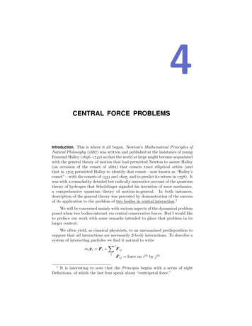
8Central force problemsx1 , x2 , x3 , x4 } that serveFigure 4a: Shown above : the vectors {xto describe the instantaneous positions of {m1 , m2 , m3 , m4 } relativeto an inertial frame. Shown below: the vector X that marks theposition of the center of mass and the vectors {rr1 , r 2 , r 3 , r 4 } thatserve—redundantly—to describe position relative to the center ofmass.
9Reduction to the equivalent 1-body problem: Jacobi coordinatesm3R3m2R4m4XR2m1Figure 4b: “Calder construction” of a system of Jacobi vectors.HereR 2 proceeds m2 m1R 3 proceeds m3 center of mass of {m1 , m2 }R 4 proceeds m4 center of mass of {m1 , m2 , m3 }.X marks the center of mass of the entire populationAlternative Jacobi systems would result if the particle names werepermuted.What he have in (8) is the description of a change of variables8 x1 , x2 , . . . , xN X , R 2 , . . . , R Nthat serves to render compliance withmi ri 0 automatic. Introduction ofRthe -variableshas permitted us to avoid the “discriminatory asymmetry” ofr1 m11 m2 r2 · · · mN rN , but at cost of introducing an asymmetry ofa new sort: a population of N masses can be “mobilized” in N ! distinct ways;to select one is to reject the others, and to introduce hierarchical order where(typically) none is present in the physics.8Through presented in the case N 4, it is clear how one would extend (8)to higher order. To pull back to order N 3 one has only to strike the firstequation and then to set m4 0 in the equations that remain.
10Central force problemsSo far as concerns the dynamical aspects of that physics, we find (withmajor assistance by Mathematica) that12 x1· ẋx2· ẋx1 m2ẋx2m1ẋ X· ẊX 12 µ2ṘR2R2· Ṙm1 m2 Ẋ 1x xx xx x2 m1 ẋ 1· ẋ 1 m2 ẋ 2· ẋ 2 m3 ẋ 3· ẋ 3 12R2 12 µ3ṘR3X· ẊX 12 µ2ṘR2· ṘR3· Ṙm1 m2 m3 Ẋ 1x xx xx xx x2 m1 ẋ 1· ẋ 1 m2 ẋ 2· ẋ 2 m3 ẋ 3· ẋ 3 m4 ẋ 4· ẋ 4 12 .12R2 12 µ3ṘR3 12 µ4ṘR4X· ẊX 12 µ2ṘR2· ṘR3· ṘR4· Ṙm1 m2 m3 m4 Ẋwhereµ2 µ3 µ4 . 1m1 1m21µ2 1m31µ3 1m4 –1 –1 –1 m1 m2m1 m2(m1 m2 )m3m1 m2 m3 (m1 m2 m3 )m4m1 m2 m3 m4 (9)serve to generalize the notion of “reduced mass.” Theterms fact that no cross appear when kinetic energy is described in terms of X , R 2 , . . . , R N variablesis—though familiar in the case N 2—somewhat surprising in the generalcase. I look to the underlying mechanism, as illustrated in the case N 3: wehave r1 r 2 M R 2R3r3 2 m1m m2 m1M m1 m2 0m3 m1 m2 m3 m3 m1 m : Note that M is 3 2 m23 1 m2 m1m m2 m3The claim—verified by Mathematica—is that m1M T 000m20 0µ2 M 00m30µ3 But while the R -variables are well-adapted to the description of kinetic energy,
Reduction to the equivalent 1-body problem: Jacobi coordinates11we see from9r1 r2 R2r1 r3 r2 r3 m2m1 m2 R 2m2m1 m2 R 21 m1m mR22r2 r4 1 m1m mR22r1 r4 r3 r4 R3 m3m1 m2 m3 R 3 R3 m3m1 m2 m3 R 3m1 m2m1 m2 m3 R 3 R4 R4 R4that R -variables are (except in the case N 2) not particularly well-adaptedto the description of (the distances which separate the masses, whence to thedescription of) central 2-body interactive forces. In the case of the graviational3-body problem we now find ourselves led to write 1 12 222U G m1 m2 R22 2 m1 m3 m1m mR2 m1m mR 2·R 3 R32 222 1 2 2m12 21 m2 m3 m1m mR R·R R2323m1 m22 Gm1 m2 / R 2·R 2 when m3 is extinguishedwhich provides one indication of why it is that the 2 -body problem is so mucheasier than the 3 -body problem, but at the same time suggests that the variablesR 2 and R 3 may be of real use in this physical application. As, apparently,they turn out to be: consulting A. E. Roy’s Orbital Motion ( ), I discoverR 2 and ρ RR 3 were introduced by Jacobi and(see his §5.11.3) that r RLagrange, and are known to celestial mechanics as “Jacobian coordinates.” Foran interesting recent application, and modern references, see R. G. Littlejohn& M. Reinseh, “Gauge fields in the separation of rotations and internal motionsin the n-body problem,” RMP 69, 213 (1997).It is interesting to note that the pretty idea from which this discussionhas proceeded (Figure 4b) was elevated to the status of (literally) fine artby Alexander Calder ( – ), the American sculptor celebrated for hisinvention of the “mobile.”9The following equations can be computed algebraically from (19). Butthey can also—and more quickly—be read off directly from Figure 4b : toj and walks along the figure to i , taking signscompute r i r j one starts at to reflect whether one proceeds prograde or retrograde along a given leg, and(when one enters/exits at the “fulcrum” of a leg) taking a fractional factorwhich conforms to the “teeter-totter principle”factional factor mass to the rear of that legtotal mass associated with that legA little practice shows better than any explanation how the procedure works,and how wonderfully efficient it is.
12Central force problems2. Mechanics of the reduced system: motion in a central force field. We studythe systemL(ṙr, r ) 12 µ ṙr · ṙr U (r)(10)x2 .where I have written r for the vector that came to us (Figure 3) as R x1 xEquivalently1H(pp, r ) 2µp · p U (r)(11)wherep L/ ṙr µ ṙrThe Lagrange equations read µr̈r U 0 or (compare (5.2))µr̈r r1 U (r) r(12)which in the Hamiltonian formalism are renderedṙr 1µp1ṗp r U (r) r(13)From the time-independence of the Lagrangian it follows (by Noether’s theorem)that energy is conservedE 12 µ ṙr · ṙr U (r)is a constant of the motion(14)while from the manifest rotational invariance of the Lagrangian it follows (onthose same grounds) that angular momentum10 is conservedL r p is a vectorial constant of the motion(15)We can anticipate that once values have been assigned to E and L the generalsolution r (t; E, L) of the equation(s) of motion (12) will contain two adjustableparameters. In Hamiltonian mechanics (14) reduces to the triviality [H, H ] 0while (15) becomes[H, L ] 0(16)Since L stands to the plane defined by r and p,11 and since also L isinvariant, it follows that the vectors r (t) are confined to a plane—the orbitalplane, normal to L, that contains the force center as a distinguished point. Theexistence of an orbital plane can be understood physically on grounds that—because the force is central—the particle never experiences a force that wouldpull it out of the plane defined by {rr(0), ṙr(0)}.10What is here called “angular momentum” would, in its original 2-bodycontext, be called “intrinsic angular momentum” or “spin” to distinguish itX ẊX : the familiar distinction here isfrom the “orbital angular momentum” MXbetween “angular momentum of the center of mass” and “angular momentumabout the center of mass.”11The case r p is clearly exceptional: definition of the plane becomesambituous, and L 0.
13Motion in a central force fieldReorient the reference frame so as to achieve 0L 0 (and install polar coordinates on the orbital plane:r1 r cos θr2 r sin θWe then haveL T U 12 µ(ṙ2 r2 θ̇2 ) U (r)(17)Time-independence implies conservation ofE 12 µ(ṙ2 r2 θ̇2 ) U (r)(18)while θ-independence implies conservation of pθ L/ θ̇ µr2 θ̇. But from L3 r1 p2 r2 p1 µ r cos θ(ṙ sin θ rθ̇ cos θ) r sin θ(ṙ cos θ rθ̇ sin θ) µr2 θ̇(19)we see that pθ , L3 and ( are just different names for the same thing. From (18)we obtain ṙ µ2 E U (r) r2 θ̇2θ̇ (/µr2which bybecomes 2µ E U (r) 2(20)(21)2µr 2This places us in position once again to describe a “time of flight” rtr0 r r01 2µ E U (r) 2 dr(22)2µr 2which by functional inversion (if it could be performed) would supply r(t).Moreover(/µr2dθ θ̇ 2 drṙ2E U (r) µ2µr 2
14Central force problemswhich provides this “angular advance” formula r(/µr2 θ θ0 2r0µ E U (r) 2 dr(23)2µr 2But again, a (possibly intractable) functional inversion stands between thisand the r(θ; E, () with which we would expect to describe an orbit in polarcoordinates.At (21) the problem of two particles (masses m1 and m2 ) movinginteractively in 3-space has been reduced to the problem of one particle (mass µ)moving on the positive half of the r -line in the presence of the effective potential2U (r) U (r) ( 22µr(24)—has been reduced, in short, to the problem posed by the effective LagrangianL 12 µṙ2 U (r)The beauty of the situation is that in 1-dimensional problems it is possibleto gain powerful insight from the simplest of diagramatic arguments. We willrehearse some of those, as they relate to the Kepler problem and other specialcases, in later sections. In the meantime, see Figure 5.Bound orbits arise when the values of E and ( are such that r is trappedbetween turning points rmin and rmax . In such cases one has θ angular advance per radial period rmax(/µr2 2dr2 2rminE U(r) 2µ2µr(25)with consequences illustrated in Figure 6. An orbit will close (and motionalong it be periodic) if there exist integers m and n such thatm θ n2πMany potentials give rise to some closed orbits, but it is the upshot of Bertrand’stheorem12 that only two power-law potentialsU (r) kr2U (r) k/r::isotropic oscillatorKepler problemhave the property that every bound orbit closes (and in both of those casesclosure occurs after a single circuit.I return to this topic in §7, but in the meantime, see §3.6 and Appendix Ain the 2nd edition ( ) of H. Goldstein’s Classical Mechanics. . Or see §2.3.3in J. V. José & E. Saletan, Classical Dynamics: A Contemporary Approach( ).12
15Motion in a central force fieldFigure 5: Graphs of U (r), shown here for ascending values ofangular momentum ( in the Keplerian case U (r) k/r (lowestcurve). When E 0 the orbit is bounded by turning points atrmin and rmax . When rmin rmax the orbit is necessarily circular(pursued with constant r) and the energy is least-possible for thespecified value of (. When E 0 the orbit has only one turningradius: rmax ceases to exist, and the physics of bound states becomesthe physics of scattering states. The radius rmin of closest approachis (-dependent, decreasing as ( decreases.Circular orbits (which, of course, always—after a single circuit—close uponthemselves) occur only when the values of E and ( are so coordinated as toachieve rmin rmax (call their mutual value r0 ). The energy E is then leastpossible for the specified angular momentum ( (and vice versa). For a circularorbit one has (as an instance of T 12 Iω 2 L2 /2I )kinetic energy T (22µr02but the relation of T to E T U (r0 ) obviously varies from case to case.But here the virial theorem13 comes to our rescue, for it is an implication ofnthat pretty proposition that if U (r) krn then on a circular orbit T 2 U (r0 )which entailsn 2n 2E n T 2 UFor an oscillator we therefore have2 22µω r0E 2· ( 2 2·2µr02 r02 (/µω E (ωWe will return also to this topic in §7, but in the meantime see Goldstein12or thermodynamics & statistical mechanics ( ), pages 162–164.13
16Central force problemsFigure 6: Typical bound orbit, with θ advancing as r oscillatesbetween rmax and rmin , the total advance per oscillation being givenby (25). In the figure, radials mark the halfway point and end ofthe first such oscillation.Figure 7: Typical unbounded orbit, and its asymptotes. The anglebetween the asymptotes (scattering angle) can be computed from(26). The dashed circle (radius rmin ) marks the closest possibleapproach to the force center, which is, of course, {E, (}-dependent.
17Orbital designwhich by the quantization rule n would giveE n ω:n 0, 1, 2, . . .Similarly, in case of the Kepler problem we have2E 2 12 ( k/r0 )2µr0 2r0 µk 2µkE 22 which upon formal quantization yields Bohr’sE µk 2 12 2 n2:n 1, 2, 3, . . .If E is so large as to cause the orbit to be unbounded then (questionsof closure and periodicity do not arise, and) an obvious modification of (25)supplies θ scattering angle /µr2 22rminE U (r) µ 22µr 2 dr(26)Even for simple power-law potentials U krn the integrals (25) and (26)are analytically intractable except in a few cases (so say the books, andMathematica appears to agree). Certainly analytical integration is certainlyout of the question when U (r) is taken to be one or another of the standardphenomenological potentials—such, for example, as the Yukawa potential λrU (r) kerBut in no concrete case does numerical integration pose a problem.3. Orbital design. We learned already in Chapter 1 to distinguish the design of atrajectory (or orbit) from motion along a trajectory. We have entered now intoa subject area which in fact sprang historically from a statement concerningorbital design: the 1st Law ( ) of Johannes Kepler ( – ) asserts that“planetary orbits are elliptical, with the sun at one focus.” We look to whatcan be said about orbits more generally (other central force laws).We had at bottom of page 13 a differential equation satisfied by θ(r). Formany purposes it would, however, be more convenient to talk about r(θ), andin pursuit of that objective it would be very much to our benefit if we could
18Central force problemsfind some way to avoid the functional inversion problem presented by θ(r). Tothat end we return to the Lagrangian (17), which suppliesdµr̈ µrθ̇2 drU (r) f (r)But at (20) we had θ̇ /µr2 , soµr̈ 2 /µr3 f (r)From (20) it follows also thatddtd ( /µr2 ) dθso we have d 1 d 3( 2 /µ) r12 dθr 2 dθ r (1/r ) f (r)Introduce the new dependent variable u 1/r and obtain 2d 2d 1 u dθ u dθ u u3 (µ/ 2 )f ( u1 )whenced 2 u u (µ/ 2 ) 1 f ( 1 )u2udθ2d U ( u1 ) (µ/ 2 )du(27.1)For potentials of the form U (r) krn we therefore have n(kµ/ 2 ) u n 1(27.2)The most favorable cases, from this point of view, are n 1 and n 2.EXAMPLE: Harmonic central potentialwhere (27.2) readsWe look to the case U (r) 12 µω 2 r2d 2 u u (µω/ )2 u 3dθ2(28)and, because our objective is mainly to check the accuracy of recent assertions, we agree to “work backwards;” i.e., from foreknowledge of the elementaryfact that the orbit of an isotropic oscillator is a centered ellipse. In standardorientationx2 y 2 1a2b2 r(θ) b2cos2a2 b2θ a2 sin2 θ
Orbital design Figure 8: Figure derived from (29), inscribed on the a, b -plane,shows a hyperbolic curve of constant angular momentum and severalcircular arcs of constant energy. The energy arc of least energyintersects the -curve at a b: the associated orbit is circular.Figure 9: Typical centered elliptical orbit of an isotropic harmonicoscillator, showing circles of radii rmax a and rmin b. Theisotropic oscillator is exceptional (though not quite unique) in thatfor this as for all orbits the angular advance per radial oscillationis θ π : all orbits close after a single circuit.19
20Central force problemsso for an arbitrarily oriented centered ellipse we have b2 cos2 (θ δ) a2 sin2 (θ δ)u(θ) a2 b2Mathematica informs us that such functions satisfy (28) with µ ωab(29.1)Such an orbit is pursued with energyE 12 µω 2 (a2 b2 )(29.2)From (29) we obtaina2 E 2 1 µω1 ωE2b2 E 2 1 µω1 ωE2Evidently circular orbits (a b) require that E and stand in the relation E ω encountered already at the bottom of page 15 (see Figure 8). Returningwith (29) to (25) we find that the angular advance per radial oscillation is givenby aab/r2 θ 2dra2 b2 r2 a2 b2 /r2b π:all {a, b}, by numerical experimentationwhich simply reaffirms what we already knew: all isotropic oscillator orbits areclosed/periodic (see Figure 9).4. The Kepler problem: attractive 1/ r 2 force. HereU (r) k r1:k 0and the orbital equation (27.2) readsd 2 u u (kµ/ 2 )u0dθ2 por againd 2v v 0dθ2Immediately v(θ) q cos(θ δ) so1p q cos(θ δ)α 1 ε cos(θ δ)with v u pr(θ) :more standard notation(30)
21The Kepler problemFigure 10: Keplerian ellipse (30) with eccentricity ε 0.8. Thecircles have radiirmin α: “pericenter”1 εrmax α: “apocenter”1 εWhen the sun sits at the central focus the “pericenter/apocenter”become the “perihelion/aphelion,” while if the earth sits at the focusone speaks of the “perigee/apogee.” It is clear from the figure, andan immediate implication of (30), that θ 2πEquation (30) provides—as Kepler asserted, as a little experimentation withMathematica’s PolarPlot[etc] would strongly suggest, and as will presentlyemerge—the polar description of an ellipse of eccentricity ε with one focus atthe force center (i.e., at the origin).To figure out how α and ε depend upon energy and angular momentumwe return to (23) which gives r 2 θ drp qr 1 r 2 1 dup qu u2 q 2u arctan 2 p qu u2 q 2u arcsin q 2 4p
22Central force problemsFigure 11: Graphs of confocal Keplerian conic sectionsr 11 ε cos θwith ε 0.75, 1.00, 1.25.where now p 2Eµ/ 2 and q 2kµ/ 2 . So we have u 12 q 12 q 2 4p sin θand have only to adjust the point from which we measure angle (θ θ 12 π)to recover (30) with (see the figure)2α 2/q µk0 ε 1 4p/q 2 21 2E 2µk 1 : ellipse 1 : parabola 1 : hyperbola(31)To achieve a circular orbit (ε 0) one must haveE µk 22 2i.e., E 2 12 µk 2which was encountered already on page 17, and which describes the least energy possible for a given angular momentum the greatest angular momentum possible for a given energyfor if these bounds were exceeded then ε would become imaginary.The semi-major axis of the Keplerian ellipse isa 12 (rmin rmax ) α 21 ε k: positive because E 02E(32.1)
23The Kepler problemwhile the semi-minor axis (got by computing the maximal value assumed byr(θ) sin θ ) is b α aα(32.2)21 ε : real for that same reason 2µEThe distance from center to focus is f ε a so the distance from focus toapocenter is (1 ε)a α/(1 ε) rmin : this little argument serves to establishthat the force center really does reside at a focal point.Concerning secular progress along an orbit: the area swept out by r is θA(θ) 12r2 (ϑ) dϑso the rate of growth of A isȦ 12 r2 θ̇ 12µ constant for every force law(33) 1Multiplication by the period τ gives 2µ τ πab πa aα whence (by (31))τ2 :4π 2 µ2 34π 2 µ 3aαa 2k(34)In the gravitational case one hasµm 1 m211· kGm1 m2 m1 m2G(m1 m2 )If one had in mind a system like the sun and its several lesser planets one mightwriteτ1 2M m2 a1 3 τ2M m1 a2and with the neglect of the planetary masses obtain Kepler’s 3rd Law ( )τ1τ22 a1a23(35)It is interesting to note that the harmonic force law would have supplied, by1the same reasoning (but use (29.1)), 2µ τ πab π /µ ω whenceτ 2π/ω:all values of E and We have now in hand, as derived consequences of Newton’s Laws of Motionand Universal Law of Gravitation, kepler’s first law of planetary motion: Planets pursue ellipticalorbits, with the sun at one focus; kepler’s second law: The radius sweeps out equal areas in equal times; kepler’s third law: For any pair of planets, the square
2 Central force problems andtowrite F ij F ji: “action reaction” (1.1) asanexpressionofNewton’s3rd Law.