Transcription
An Introduction to Extreme Value StatisticsMarielle Pinheiro and Richard Grotjahn
iiThis tutorial is a basic introduction to extreme value analysis and the R package, extRemes. Extreme valueanalysis has application in a number of different disciplines ranging from finance to hydrology, but here theexamples will be presented in the form of climate observations.We will begin with a brief background on extreme value analysis, presenting the two main methods andthen proceeding to show examples of each method. Readers interested in a more detailed explanation of themath should refer to texts such as Coles 2001 [1], which is cited frequently in the Gilleland and Katz extRemes2.0 paper [2] detailing the various tools provided in the extRemes package. Also, the extRemes documentation,which is useful for functions syntax, can be found at tRemes.pdfFor guidance on the R syntax and R scripting, many resources are available online. New users might want tobegin with the Cookbook for R (http://www.cookbook-r.com/ or Quick-R (http://www.statmethods.net/)
Contents1 Background1.1 Extreme Value Theory . . . . . . . . . . . . . . . . . . . . . . . . . . . . . . . . . . . . . . . . . .1.2 Generalized Extreme Value (GEV) versus Generalized Pareto (GP) . . . . . . . . . . . . . . . . .1.3 Stationarity versus non-stationarity . . . . . . . . . . . . . . . . . . . . . . . . . . . . . . . . . . .2 ExtRemes example: Using Davis station data from 1951-20122.1 Explanation of the fevd input and output . . . . . . . . . . . . . . . . . .2.1.1 fevd tools used in this example . . . . . . . . . . . . . . . . . . . .2.2 Working with the data: Generalized Extreme Value (GEV) distribution fit2.3 Working with the data: Generalized Pareto (GP) distribution fit . . . . .2.4 Using the model fit: probabilities and return periods . . . . . . . . . . . .2.4.1 The relationship between probability and return period . . . . . .2.4.2 Test case: 2013 and 2014 records . . . . . . . . . . . . . . . . . . .2.4.3 Comparing model probabilities and return periods . . . . . . . . .2.4.4 Comparing empirical probabilities and return periods . . . . . . .2.4.5 Results: comparing empirical versus model return periods . . . . .2.5 Discussion: GEV vs. GP . . . . . . . . . . . . . . . . . . . . . . . . . . . .2.5.1 How well does each method capture the data distribution? . . . . .2.5.2 How do the results from each method compare to one another? . .1123778910111112131313131314Appendix A Explaining fevd output17A.1 fevd output . . . . . . . . . . . . . . . . . . . . . . . . . . . . . . . . . . . . . . . . . . . . . . . . 17A.2 Other fevd options . . . . . . . . . . . . . . . . . . . . . . . . . . . . . . . . . . . . . . . . . . . . 18Appendix B GP fittingB.1 Threshold selection . . . . . . . . . .B.2 Declustering data . . . . . . . . . . .B.3 Nonstationary threshold calculationB.3.1 Sine function . . . . . . . . .B.3.2 Harmonics function . . . . .191920222222Appendix C Some R syntax examplesC.1 Installing and running R . . . . . .C.1.1 Installing R . . . . . . . . .C.1.2 Running R . . . . . . . . .C.1.3 Installing Packages . . . . .C.2 Formatting text files . . . . . . . .C.3 Reading and subsetting data in R .C.3.1 Some user-defined functionsC.4 Plots . . . . . . . . . . . . . . . . .252525252526272729.iii
ivCONTENTS
Chapter 1Background1.1Extreme Value TheoryIn general terms, the chance that an event will occur can be described in the form of a probability. Think of acoin toss; in an ideal scenario, there is a 50% chance that the coin will land either heads or tails up in a singletrial, and as multiple tosses are made, we gather additional information about the probability of landing onheads versus tails. With this knowledge, we can make predictions about the outcomes of future trials.The coin toss scenario is an example of a simple binomial probability distribution (frequency of headsversus frequency of tails), but the fundamental concept can be expanded to encompass more complex scenarios,described by other probability distributions. Here, we are interested in formulating a mathematical representation of extremes, or events with a low probability of occurrence. The definition of extremes varies by fieldand methodology; in the context of climate, we will talk about extreme temperatures, such as the higher-thanaverage temperatures experienced over the course of a heat wave. An extreme weather event is an occurrencethat deviates substantially from typical weather at a specific location and time of year. Specific definitionsvary depending on the distribution of local weather patterns and method of categorization. Analysis of extremeweather is made more difficult by the fact that extreme events are, by definition, rare, and therefore reliabledata is limited.Extreme value theory deals with the stochasticity of natural variability by describing extreme events withrespect to a probability of occurrence. The frequency of occurrence for events with varying magnitudes can bedescribed as a series of identically distributed random variablesF X1 , X2 , X3 , .XN(1.1)where F is some function that approximates the relationship between the magnitude of the event (variableXN ) and the probability of its occurrence.While it is possible to do analysis with the overall distribution of temperature magnitudes, we are focusing onjust the extreme temperatures, which can also be described in terms of a probability distribution function. Wecan use the information from the resultant distribution to analyze trends and the likelihood that catastrophicevents will occur. Here are just a few of the possibilities: Predict how often catastrophic events are likely to occur (return level)– extreme temperatures (heat waves, cold air outbreaks)– precipitation levels, flooding and droughts– hurricane frequency and magnitude Perform simulations utilizing the distributions, and use the results to anticipate future concerns– How does the occurrence of current temperatures match the calculated probability of occurrence? Ina changing climate, what can we expect to change in terms of temperature trends?– What do current precipitation levels mean for reservoir levels and overall water usage?– What changes can we expect for the intensity and frequency of hurricanes?1
2CHAPTER 1. BACKGROUND1.2Generalized Extreme Value (GEV) versus Generalized Pareto(GP)We will focus on two methods of extreme value analysis. The first approach, GEV, looks at distribution ofblock maxima (a block being defined as a set time period such as a year); depending on the shape parameter,a Gumbel, Fréchet, or Weibull1 distribution will be produced. The second method, GP, looks at values thatexceed a defined threshold2 ; depending on the shape parameter, an Exponential, Pareto, or Beta distributionwill be produced.The two methods are summarized below; a demonstration of each method follows in the next chapter.GEVDistribution function of standardized maxima (or minima)— block maxima/minimaapproachlocation µ: position of the GEV meanDescriptionParametersGeneral function (CDF)Limit as ξ 0threshold u : Reference value for whichGP excesses are calculatedscale σ: multiplier that scales functionshape ξ: Parameter that describes the relative distribution of the probabilities.for extreme value z,for threshold excess x," # 1/ξ 1/ξx uz µH(x) 1 1 ξG(z) exp 1 ξσuσ Gumbel:ξ 0ξ 0Interpretation of resultsGPprobability of exceeding pre-determinedthreshold— peaks over threshold approachExponential: z µG(z) exp exp σ x uH(x) 1 exp σFréchetWeibullReturn level: value zp that is expected tobe exceeded on average once every 1/p periods, where 1 p is the probability associated with the quantile. Find zp such thatG(zp ) 1 pParetoBetaReturn level: value xm that is exceededevery m times. Begin by estimating ζu ,the probability of exceeding the threshold.Then, xm is u σξu [(mζu )ξ 1] ξ 6 0xm u σu ln(mζu )ξ 0Table 1.1: Description of the two basic types of extreme value distributionsProbability density functions (PDFs) and cumulative distribution functions (CDFs)The probability density function (as shown in Figure 1.1), plots the relative likelihood (on the yaxis) that a variable will have value X (on the x axis). Contrast this with the cumulative distributionfunction (as shown in Figure 1.2), in which the probability of X is defined by integrating the PDF overthe range in which the variable X. Note that the equations in Table 1.1 are CDFs, not PDFs.1 Notethat the Weibull distribution has a finite right endpoint; Gumbel and Fréchet have infinite right endpointsGP function can be approximated as the tail of a GEV; the scale parameter σu is a function of the threshold and isequivalent to σg ξ(u µ), where σg , ξ and µ are all parameters of a corresponding GEV distribution2 The
1.3. STATIONARITY VERSUS NON-STATIONARITY3Figure 1.1: Probability density functions for (left) GEV and (right) GP. For each plot, x and µ 1, σ 0.5. Forξ, blue -0.5, black 0, and red 0.5Figure 1.2: Cumulative density functions for (left) GEV and (right) GP. For each plot, x and µ 1, σ 0.5. Forξ, blue -0.5, black 0, and red 0.51.3Stationarity versus non-stationarityIn calculating the model fit, it is useful to determine whether the model distribution remains the same as timeprogresses. Figure 1.3 shows how the probability of the extremes might change in the future under possibleproposed climate scenarios. Note that the model that was fit to an extreme temperature distribution from the20th century might not work for 21st century values.Figure 1.3: Temperature magnitudes and probability of occurrence in the context of a warmer climate. Plotsobtained from IPCC Summary for Policymakers (2012), Figure SPM.3This change can be incorporated into the model as a change with respect to time; µ, x, σ, and ξ can berepresented as some sort of function of time. This is known as a non-stationary model, in contrast to astationary model in which the model parameters are fixed constants.For example, if we anticipated that there would be a greater proportion of extreme high temperatures in thefuture, the shape of a GEV function fitted to the data might increase towards a more heavy-tailed distribution,as seen in Figure 1.4.
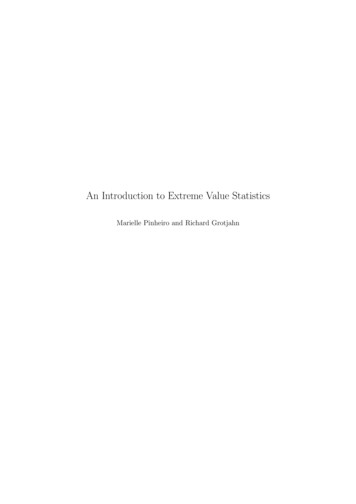
4CHAPTER 1. BACKGROUNDFigure 1.4: Altering ξ in a GEV distribution as a function of time: ξ(t) 0.02t. Black: t 0 Green: t 15Purple: t 50. Other parameters remain constant.Non-stationarity is most often seen with GP distributions where the threshold is defined as a function. Ifwe wanted to increase the GP threshold linearly, as might be the case in an increasingly warmer climate, wecould define the threshold asx(t) x0 x1 t(1.2)where x0 would be the initial threshold value and x1 would increment the threshold value over time. Thesame can be done for the other parameters as well; for example,The parameters could also be tailored to incorporate some sort of seasonal cycle; Figure 1.5 demonstratesthat there is a definite trend to the temperature values throughout the JJAS months, so we tailor the thresholdaccordingly by writing the threshold as a sine function (see Appendix B.3.1 for equation). Note the differencein the number of points that exceed the non-stationary threshold (red) as opposed to the stationary threshold(blue). We gain some points in June and September, and lose some points in July and August.Another method, which will be used in this study (see section 2.3 for a demonstration), utilizes the value ofthe 90th percentile for each day in the season to provide an initial estimate for a threshold value, and then fitsa sum of sines and cosines to those estimates; this is known as a sum of harmonics. The 90th percentile valuesare plotted on Figure1.6 as the green line, with the corresponding harmonics sum plotted in black. At manyspots throughout the season, the black line is reasonably close to the sine function, but there are notable dipsin mid-August and mid-September.Figure 1.7 demonstrates how the distribution of the excesses changes with each of the methods. Altering theshape of the threshold also changes the magnitude of the excesses, and this leads to a different GP distribution,highlighting the importance of choosing a proper threshold.Limitations of non-stationary threshold in extRemesCertain methods in the extRemes package will be unavailable when using a non-stationary threshold;for example, threshrange.plot, which is used to determine an optimal threshold value, will not workwith a non-constant threshold. If you are going to use a non-stationary threshold, it is suggested thatyou begin by making an initial constant threshold estimate using threshrange.plot. Then, examinethe data for any possible time-dependent trends and determine a threshold function that is near to theinitial constant threshold. Finally, calculate a new dataset with threshold excesses as demonstrated inSection 2.3
1.3. STATIONARITY VERSUS NON-STATIONARITY5Figure 1.5: Daily maximum temperatures from 1951-2012, plotted with respect to day in season. Blue linerepresents a constant threshold of 37, while red line represents a threshold with equation B.2, which is a sinefunction intended to follow the seasonal trend. Vertical lines denote division of months.Figure 1.6: Modification of Figure 1.5 to show newly calculated threshold based on fitting harmonic equation to90th percentile values. Sine function in red, 90th percentile values in green, fitted harmonics equation in black
6CHAPTER 1. BACKGROUNDFigure 1.7: A comparison of the GP PDFs for (top) a constant threshold of 37, (middle) a sine-varying threshold,and (bottom) a harmonics-fitted threshold. Black solid lines represent the probabilities of the excesses as relatedto the various thresholds, and blue dashed lines represent the PDF that was calculated by extRemes based onthe excesses.
Chapter 2ExtRemes example: Using Davisstation data from 1951-2012Now we will turn to the application of each distribution function and interpret the results. This chapter willfocus on two main questions:1. How well does each method capture the data distribution?2. How do the results from each method compare to one another?Before you begin:See Appendix C.1 for instructions on how to install and run R, if you haven’t already done so. TheextRemes library must also be installed.Appendix C.3 contains some useful tips for subsetting and processing datasets in preparation for usewith extRemes.2.1Explanation of the fevd input and outputThe fevd function is the primary function in the extRemes package; it calculates the parameters for the specifiedprobability distribution that best fits the data, and all other calculations are based off of this fit. See AppendixA for definitions of the various statistical parameters in the fevd output.The syntax for fevd in this example isfevd(data, type, units, span, time.units, threshold.)1Usage:1. data: Dataset. Make sure that your data is appropriate for the calculation method– block maximarequires a single maximum (or minimum) value per block of time (e.g. per year), as opposed to peaksover threshold, which requires all of the daily maxima per length of time being analyzed (in this case, thesummer seasons for the 51-year time span).2. type: specify "GEV" or "GP"3. units: Units of dataset (here, "deg C"). Optional.4. span: defines the number of years in the model (necessary for GP model)5. time.units: Only needed if span is undefined; determines the number of years in the data. Here, we arelooking at the summer months; the number of days is 122 (30 for June, 31 for July, 31 for August, 30 forSeptember) so time.units "122/year"6. threshold: Only necessary for GP method. This is the value x from which excesses are calculated.Appendix B explains how to determine an appropriate threshold.1 there are additional options beyond the ones specified here, but for the purposes of this example we are sticking to the simplest models; check the extRemes documentation for more extensive functionality7
8CHAPTER 2. EXTREMES EXAMPLE: USING DAVIS STATION DATA FROM 1951-20122.1.1fevd tools used in this example plot.fevdSyntax: plot(fit,type.)Usage: The default plot(fit) with only the fit variable (your fevd variable) as an argument will returna 4-plot figure with:1. Top left (type "qq"): Quantile-quantile plots, with model quantiles on the x axis and empiricalquantiles on the y axis and a black line representing the 1-1 line.2. Top right (type "qq2"): Quantile-quantile plots, with empirical quantiles on the x axis, modelquantiles on the y axis, and confidence intervals as dashed grey lines. The 1-1 line is drawn as anorange dashed line and the linear fit of the quantile-quantile plot is drawn as a solid grey line.3. Bottom left (type "density"): Model (dashed blue line) and observational data (solid black line)PDFs4. Bottom right (type "rl"): Plot of the return period in years (x axis) for various temperaturemagnitudes (y axis)Figure 2.1: Default output for plot.fevd (shown for GEV model). This is type "primary".If you wish to output only a single plot, or a plot that’s not one of the defaults, specify the type("probprob", "qq", "qq2", "Zplot", "hist", "density", "rl", "trace")
2.2. WORKING WITH THE DATA: GENERALIZED EXTREME VALUE (GEV) DISTRIBUTION FIT 9 pextRemes.fevd: the probability of fit q, where q is a vector of specified values q c(num1,num2.)Syntax: pextRemes(fit, q, lower.tail FALSE,.) rextRemes.fevd: Create simulated data sets based on the calculated probability distribution, where n isthe number of random draws.Syntax: rextRemes(fit, n,.) ci.fevd: the confidence interval associated with either the fit parameters (ci(fit,type "parameter"))or estimated n-year return period temperature value (ci(fit,type "return.level",return.period n)).Syntax: ci(fit,type,return.period,.)2.2Working with the data: Generalized Extreme Value (GEV) distribution fitOur dataset, shown in Figure 2.2, is the 1951-2012 maximum recorded temperature (in degrees Celsius) for themonths June, July, August, and September per year from an observation station based in Davis, California.There are 62 data points, one for each 122-day period per year.Figure 2.2: Seasonal maximum temperature for JJAS per year at Davis station, 1951-2012Let us begin with some initial observations. Using summary(davis max), we getMin. 1st Qu.37.7840.69Median41.67Mean 3rd Qu.41.6142.64Max.45.00There is an average maximum value of 41.61 degrees Celsius with the greatest maximum being 45 degrees Celsius for the 62-year period. Figure 2.3, generated using plot(fit1,type "density") and plot(fit1,type "qq2"),shows the PDF generated by the model against the actual distribution of block maxima.We can examine the confidence interval of the parameters as follows:ci(fit1,type "parameter")fevd(x davis max, type "GEV", units "deg C")[1] "Normal Approx."locationscaleshape95% lower CIEstimate 95% upper CI40.7374923 41.124273341.51105421.1735853 1.43489181.6961983-0.4124608 -0.2902778-0.1680947How well does the GEV method capture the data distribution?Based just on observing the calculated PDF versus empirical data PDF, the model seems to have a reasonablygood fit for most of the data, and the confidence intervals for the parameters reflect this.
10CHAPTER 2. EXTREMES EXAMPLE: USING DAVIS STATION DATA FROM 1951-2012Figure 2.3: Left: Model distribution (blue dashed line) vs actual temperature probability distribution (blacksolid line) Right: Quantile-quantile plot with empirical quantiles on the x-axis and model quantiles on they-axis2.3Working with the data: Generalized Pareto (GP) distributionfitIn the GP example, we will use the data from the same observation station, but the dataset is extended toinclude all recorded daily maximum temperatures for the summer months from 1951-2012, for a total of 7564data points. Using summary(davis temps), we getMin. 1st Qu.14.4429.44Median32.78Mean 3rd Qu.32.5235.56Max.45.00We calculate a new data set, excess, in which the time-varying threshold is subtracted from the temperaturevalues. Both the original temperature values and the calculated excesses can be seen in Figure 2.4. We noted inSection 1.3 that while the sine-varying threshold is pretty good at capturing the seasonal trend, the harmonicsmethod is best at matching seasonal fuctuations, and this is the one that will be used. To see how the sine andharmonics functions were calculated, refer to Appendix B.32 .We utilize a threshold of 0 when calculating the model fit. Some statistics for the distribution of temperatureexcesses:summary(excess[excess 0])Min. 1st Qu.MedianMean 3rd Qu.Max.0.005552 0.505700 1.275000 1.562000 2.317000 6.329000Figure 2.5 shows a comparison of the empirical threshold excesses with the model prediction.The confidence interval for scale and shape are shown below (threshold is excluded because it was explicitlyprovided in the function input).ci(fit2,type "parameter")fevd(x excess, threshold 0, type "GP", span 62, units "deg C",time.units "122/year")[1] "Normal Approx."scaleshape95% lower CIEstimate 95% upper CI1.8149661 1.97701372.1390613-0.3180036 -0.2693377-0.2206717How well does the GP method capture the data distribution?The selection of the harmonics-fitted threshold results in a data distribution that closely fits the calculatedGP model, with the exception of the highest extremes at the tail (as with the GEV model). Both the scale andshape parameters have small standard errors.2 AppendixB also discusses declustering, but for simplicity’s sake, we will omit declustering in this example.
2.4. USING THE MODEL FIT: PROBABILITIES AND RETURN PERIODS11Figure 2.4: Left: Daily maximum temperatures for JJAS per year at Davis station, 1951-2012. Right: Dailytemperature excesses for JJAS per year at Davis station, 1951-2012.Figure 2.5: Left: Model distribution (blue dashed line) vs actual temperature excesses (black solid line). Right:Quantile-quantile plot with empirical temperature excesses on the x-axis and model quantiles on the y-axis2.4Using the model fit: probabilities and return periodsBased on the model fits, what is the predicted return period for various return levels? Here, we compare GEVand GP outputs.2.4.1The relationship between probability and return periodFor the GEV method, there is an inverse relationship between probability and return period.3 Therefore, thereturn period for temperature magnitude z is simply defined as1(2.1)pFor the GP function, the return period calculation is complicated by the fact that there is a varying threshold.We cannot simply invert the probability for excess x, since that probability changes (as opposed to the GEVmethod, where there is a single values per year).Since the extRemes package does not have a function for calculating return period from specified returnlevel, we must estimate from a few return.level outputs. The method is:rp(z, p) 1. Create a vector of return levels for a specified range of test return periods2. find the return level with a corresponding return period that most closely matches the desired returnperiodThis is illustrated below for an example in which we are trying to find the return period for a temperatureexcess of 5 degrees Celsius.3 Note the usage of lower.tail FALSE. Recall from Table 1.1 that when calculating return period, we use the equation G(z ) p1 p; therefore, if we omit lower.tail FALSE, we will get the values for 1 p, rather than p.
12CHAPTER 2. EXTREMES EXAMPLE: USING DAVIS STATION DATA FROM 1951-2012#Generate a sequence of test return periodsy -seq(4,7,0.000001)#calculate the return levels that correspond to the return periodsrl -return.level(fit2,y)#Find the intersection of the desired value and the generated sequence of return levelsrl[rl 4.9999999 & rl 5.0000001]#This returns:5.276114 5.27611555So a return level of 5 degrees excess has a return period of approximatedly 5.28 years.2.4.2Test case: 2013 and 2014 recordsFrom records kept at the UC Davis climate station (temperatures converted from Fahrenheit to Celsius forconsistency’s sake), accessed at imate-station/,we can calculate both seasonal maxima and daily temperature excesses, and compare the predicted probabilitiesto the empirical results.For GEV calculations, we are concerned with the seasonal maxima, which, in this context, are the maximumsummer temperatures for JJAS in 2013 and 1September4040.6Table 2.1: JJAS observed maximum temperatures for Davis in 2013 and 2014Therefore, for 2013, the seasonal maximum would be 45.6 and for 2014, the seasonal maximum would be42.2.For GP calculations, we will compare the predicted probability of exceeding the threshold with the full datasets for JJAS of 2013 and 2014, also obtained from the UC Davis climate station site (shown in Figure 2.6).We can use the same threshold excess calculation function used to generate the model fit dataset to calculatethe excesses for 2013 and 2014, as shown in Figure 2.7.Figure 2.6: Daily temperature maxima for 2013 and 2014 with non-stationary thresholdFigure 2.7: Temperature excesses for 2013 and 2014
2.5. DISCUSSION: GEV VS. GP13Here are the statistics for 2013 and 2014 threshold excesses:2013:Min. 1st Qu.0.2180 0.7003Median1.8970Mean 3rd Qu.2.3280 3.0290Max.6.93002014:Min. 1st Qu. MedianMean 3rd Qu.Max.0.06429 1.14800 2.12600 2.04700 2.58000 5.044002.4.3Comparing model probabilities and return periodsIn order to directly compare the outcomes of the two methods, we will focus on the 2013 and 2014 seasonalmaxima and their probabilities, and then look at the GP-calculated probabilities in terms of the excess abovethe threshold for these same data points. The results are shown in Table 2.2.2.4.4Comparing empirical probabilities and return periodsFor the dataset which corresponds to the GEV model, the empirical probability is merely the fraction of thedata which meets or exceeds the specified return level, and the return period is the inverse of the probability: rp(Z) npoints Znyears 1The method for calculating the empirical return periods for the data which corresponds to the GP model isvery similar to the GEV method, with the added parameter of number of days: rp(X) 2.4.5npoints Xnyears ndays 11ndaysResults: comparing empirical versus model return periodsYear20132014GEV45.642.2Model RP3378.152.86Emp. RP642.29GP6.923.58Model RP3097.92 1Emp. RP640.98Table 2.2: Maxima for 2013 and 2014 and the corresponding GEV probabilities and return periods (in years);and the same data points as threshold excesses, with the corresponding GP probabilities and return periods.To summarize: 2013: For a temperature magnitude of 45.6 degrees Celsius (6.92 degrees excess above threshold), theGEV function predicts that the return period is 3378 years, while the GP function predicts that thereturn period is 3098 years. In both cases, the empirical return period for each dataset was 64 years. 2014: For a temperature magnitude of 42.2 degrees Celsius (3.58 degrees excess above threshold), the GEVfunction predicts that the return period is 3 years, while the GP function predicts that the return periodis less than a year. The corresponding empirical return periods are fairly close to the model predictions.Figure 2.8 shows the return level plots for the GEV and GP functions, respectively, with the 2013 and 2014data overlaid as colored points.2.5Discussion: GEV vs. GPThis chapter has focused on two main questions, outlined at the beginning of the chapter.2.5.1How well does each method capture the data distribution?In both the GEV and GP calculations, the empirical and model data showed good agreement with low- to midlevel extremes (in the GEV case, temperature magnitudes below 44 degrees Celsius; in the GP case, excessesless than 6 degrees Celsius). This makes sense considering that with the truly extreme extremes, they havedisproportionate representation in the data. The empirical return period of 64 years for the 2013 maximum
14CHAPTER 2. EXTREMES EXAMPLE: USING DAVIS STATION DATA FROM 1951-2012Figure 2.8: Left: GEV return periods and return levels. The red dot signifies the 2013 empirical data, while theblue dot signifies the 2014 empirical data. Right: GP return periods and return levels. The red dot signifiesthe point that corresponds to the 2013 maximum; the 2014 maximum falls outside of the plot window range.Other points from 2013 are plotted in green; other points from 2014 are plotted in purple.1, but if we obtained a larger dataset in which 45.6 temperature magnitude in this instance is the inverse of 641Celsius was still the lone extreme outlier, the return period could be much larger, like 100 years ( 100) or more.When it came to these extreme outliers, however, it’s interesting to note that the GEV model seems to doworse than the GP model for the estimating 2013 maximum value’s return period (see Figure 2.8 and the redpoint); although both methods estimate a return period of approximately 3000 years, the point falls outside ofthe GEV model’s 95% confidence interval.In both cases, the shape parameter was negative, meaning that the extremes with lesser magnitudes havea higher p
The probability density function (as shown in Figure 1.1), plots the relative likelihood (on the y axis) that a variable will have value X(on the x axis). Contrast this with the cumulative distribution functio