WIXLIB

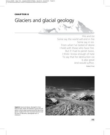
Comp. by: PG2693 Stage : Proof ChapterID: 9780521519786c08 Date:18/1/10 Time:20:56:2901 CUP/3B2/Anderson&Anderson c08.3dFilepath:H:/Glaciers and glacial geologyPolar Case0 CicedT/dz 20 C/kmdT/dz 25 C/kmTemperate Case0 CicedT/dz –0.64 C/kmdT/dz 25 C/kmFigure 8.3 Temperature profiles in polar (top) and temperate(bottom) glacier cases. Slight kink in profile in the polar casereflects the different thermal conductivities of rock and ice.Roughly isothermal profile in the temperate case is allowed bythe downward advection of heat by melt water. Temperature iskept very near the pressure-melting point throughout, meaningit declines slightly (see phase diagram of water, Figure 1.2).processes that would otherwise attack it. How does atemperate glacier remain close to the melting pointthroughout, being almost isothermal? Recall that associated with the phase change of water is a huge amountof energy. In a temperate glacier, significant watermelts at the surface, and is translated to depth withinthe firn, and even deeper in the glacier along three-grainintersections. Glacier ice is after all a porous substance.If this water encounters any site that is below thefreezing point, it will freeze, yielding its energy, whichin turn warms up the surrounding ice. So heat is efficiently moved from the surface to depth by movingwater – it is advected. This is a much more efficientprocess of heat transport than is conduction, and canmaintain the entire body of a glacier at very near thefreezing point.A straightforward distinction can be made in termsof size. Valley glaciers occupy single valleys. Ice capscover the tops of peaks and drain down severalvalleys on the sides of the peak. Ice sheets can existin the absence of any pre-existing topography, andcan be much larger by orders of magnitude than icecaps. The greatest contemporary examples are the icesheets of east and west Antarctica, and of Greenland,with diameters of thousands of kilometers, and thicknesses of kilometers. Their even larger relatives in thelast glacial maximum (LGM), the combined Laurentide and Cordillera, and the Fennoscandian IceSheets, covered half of North America and half ofEurope, respectively.Tidal glaciers are those that dip their toes in thesea, and lose some fraction of their mass throughthe calving of icebergs (as opposed to loss solelyby melting). These are the glaciers of concern toshipping, be it the shipping plying the waters ofthe Alaskan coastline, or the ocean liners plying thewaters off Greenland.Most glaciers obey what we mean when we usethe adjective “glacial.” Glacial speeds might be afew meters to a few kilometers per year, and will bethe same the next year and the next. We speak ofglacial speeds as being slow and steady. The exceptions to this are surging glaciers and their cousinsembedded in ice sheet margins, the ice streams, whichappear to be in semi-perpetual surge. These illbehaved glaciers (meaning they don’t fit our expectations) are the subjects of intense modern study. Theymay hold the key to understanding the rapid fluctuations of climate in the late Pleistocene, which in turnare important to understand as they lay the contextfor the modern climate system that humans are modifying significantly.All of these we will visit in turn, but first let us layout the basics of how glaciers work.Mass balanceThe glaciological community, traditionally an intimate mix of mountain climbers and geophysicists, hasa long and proud tradition of being quite formal inits approach to the health of glaciers and theirmechanics. Once again, the problem comes down toa balance, this time of mass of ice. One may find inthe bible of the glaciologists, Paterson’s The Physicsof Glaciers, now in its third edition (Paterson, 1994),at least one chapter on mass balance alone (seeFurther reading in this chapter for more suggestionsof other excellent textbooks). One may formalize the216

Comp. by: PG2693 Stage : Proof ChapterID: 9780521519786c08 Date:18/1/10 Time:20:56:3001 CUP/3B2/Anderson&Anderson c08.3dFilepath:H:/Mass balanceillustration of the mass balance shown in Figure 8.2with the following equation:5000@H1 @Q¼ bðzÞ @tWðzÞ @x4000Elevation (m)where H is ice thickness, W is the glacier width, and Qthe ice discharge per unit width [¼ L2/T]. Mass canbe lost or gained through all edges of the block wehave depicted (the top, the base, and the up- anddown-ice sides). Here b represents the “local massbalance” on the glacier surface, the mass lost orgained over an annual cycle. It is usually expressedas a thickness of ice surface, i.e., meters of waterequivalent. This quantity is positive where there is anet gain of ice mass over an annual cycle, and negative where there is a net loss. The elevation at whichthe mass balance crosses zero defines the “equilibrium line altitude,” or the ELA, of the glacier.Because it is an altitude, it is a horizontal line inFigure 8.2. The mass balance reflects all of themeteorological forcing of the glacier, both the snowadded over the course of the year, and the lossesdealt by the combined effects of ablation (melt) andsublimation. Where the annual mass balance is positive, it has snowed more than it melts in a year, andvice versa. To first order, because it snows more athigher altitudes, and melts more at lower altitudes,the mass balance always has a positive gradient withelevation. Examples of mass balance profiles from avariety of glaciers in differing climates are shown inFigure 8.4. Note the positive mass balance gradientin each case, which is especially well marked in theablation or wastage zones. One can easily pick outthe ELA for each glacier. The ELA varies greatly,being lowest in high latitudes (where it is cold and theablation is low) and nearest coastlines (where thewinter accumulation is high due to proximity ofoceanic water sources). A classic illustration of thelatitudinal dependence is drawn from work of Porteret al., reproduced in Figure 8.5. The modern ELAs,as deduced from snowlines and mass balancesurveys, are everywhere much higher than the ELAsreconstructed (more on how to do this later; seeFigure 8.19) from the last glacial maximum (LGM)at roughly 18 ka. In places the rise in ELA is up to1 km!One may measure the health of a glacier by thetotal mass balance, reflecting whether in a given yearthere has been a net loss or gain of ice from the te0–8–4Devon04Mass Balance (m/yr)Figure 8.4 Specific mass balance profiles from severalglaciers around the world, showing the variability of the shapeof the profiles. Mass balance gradients (slopes on this plot) arequite similar, especially in ablation zones (where the local balanceb 0), except for those in the Canadian Arctic (Devon and Whiteice caps). (adapted from Oerlemans and Fortuin, 1992, Figure 1,with permission of the American Association for the Advancementof Science)7ArcticOceanAlaskaBCCAWA OR6AlaskaRangeSt Elias5Coast CascadeRange RangeElevation 090last glacialmaximum807060504030Latitude (degrees)Figure 8.5 Profiles of topography (gray), equilibrium lineelevation (ELA, top) and glacial extent (bottom) (solid, presentday; dashed, last glacial maximum (LGM)) along the spine ofWestern North America from California to the Arctic Ocean. Notethe many-hundred meter lowering of the ELA in the LGM, andthe corresponding greater extent of the glacial coverage of thetopography. (after Skinner et al., 1999, with permission fromJohn Wiley & Sons)217

Comp. by: PG2693 Stage : Proof ChapterID: 9780521519786c08 Date:18/1/10 Time:20:56:3101 CUP/3B2/Anderson&Anderson c08.3dFilepath:H:/Glaciers and glacial geology(a)Nigardsbreen, Norway1998(b)2000summerbalance1800Elevation 00Qx1000winterbalance800u(z)Qx dxHdx600400200–12 –10 –8 –6 –4 –2 0 2Specific balance (m)Us4–40 –30 –20 –10 0Volume balance (x106m3)Figure 8.6 Mass balance profiles for the year 1998 on theNigardsbreen, a coastal Norwegian glacier. (a) Specific balancein meters of water equivalent. Winter balance from snow probesurveys, summer balance from stake network (circles). Net balanceis shown in gray; net balance is zero at 1350 m, which is the ELA.(b) The volume balance derived by the product of the specificbalance with the altitudinal distribution or hypsometry of theglacier. That the glacier has so much more area at high elevationsis reflected in the high contribution of accumulation to the netbalance of the glacier (gray fill). In 1998, the net balance ishighly positive; there is more gray area to the right of the0 balance line than to the left), so that the integral of the grayfill is 0. In this year the positive total balance representsa net increase of roughly 1 m water equivalent over theentire glacier. (after data in Kjøllmoen, 1999)glacier. This is simply the spatial integral of the product of the local mass balance with the hypsometry(area vs. elevation) of the valley:zmaxðB¼bðzÞWðzÞdzUdef10 20 30 40ð8:2Þ0This exercise is carried out annually on numerousglaciers worldwide. See Figure 8.6 for an examplefrom the Nigardsbreen, Norway. The Norwegiansare interested in the health of their glaciers becausethey control fresh water supplies, but also becausea significant portion of their electrical power comesfrom subglacially tapped hydropower sources.It is a common misconception that a considerable amount of melting takes place at the base of aglacier, because after all the Earth is hot. Note thescales on the mass balance profiles. In places, manymeters can be lost by melting associated with solarradiation. Recall that the heat flux through theEarth’s crust is about 41 mW/m2 (defined as oneheat flow unit, HFU), a trivial flux when contrastedwith the high heat fluxes powered in one or anotherFigure 8.7 (a) Mass balance for a section of glacier of width W,down-glacier length dx, and height H. Inputs or outputs throughthe top of the box dictate the local mass balance, b. Downglacierdischarge of ice into the left-hand side of the box, Qx, and out theright-hand side, Qx þ dx, include contributions from basal sliding(shading) and internal ice deformation. (after MacGregor et al.,2000, Figure 2)way by the sun (about 1000 W/m2). The upwardheat flux from the Earth is sufficient to melt about5 cm of ice per year. As far as the mass balance ofa glacier is concerned, then, there is little melt atthe base.If nothing else were happening but the local massgain or loss from the ice surface, a new lens of snowwould accumulate, which would be tapered off bymelt to a tip at the ELA (or snowline) each year. Eachsuccessive wedge would thicken the entire wedgeof snow above the snowline, and would increase theslope everywhere. But something else must happen,because we find glaciers poking their snouts wellbelow the ELA, below the snowline. How does thishappen? Ice is in motion. This is an essential ingredient in the definition of a glacier. Otherwise we aredealing with a snowfield. The Q terms in the massbalance expression reflect the fact that ice can movedownhill, powered by its own weight. Ice has twotechnologies for moving, one by basal sliding, inwhich the entire glacier moves at a rate dictated bythe slip at the bed, the other by internal deformation,like any other fluid (see Figure 8.7). We will return toa more detailed treatment of these processes in a bit.Know for now that the ice discharge per unit width ofglacier, Q, is the product of the mean velocity of the and the thickness of the glacier, H.ice column, U,Given only this knowledge, we can construct amodel of a glacier in steady state, one in which noneof the variables of concern in the mass balanceexpression are changing with time. Setting the218

Comp. by: PG2693 Stage : Proof ChapterID: 9780521519786c08 Date:18/1/10 Time:20:56:3301 CUP/3B2/Anderson&Anderson c08.3dFilepath:H:/Ice deformationIce thickness (m)20015010050001000 2000 3000 4000 5000 6000 7000 8000 9000Distance (km)01000 2000 3000 4000 5000 6000 7000 8000 9000Elevation (m)200018001600140012001000800Distance (km)Figure 8.8 Model of glacier evolution on bedrock profile fromBench Glacier valley, Alaska, shown in evenly spaced time stepsout to 600 years. Climate is assumed to be steady, with a prescribedmass balance profile. top: profiles of ice thickness through time.bottom: glacier draped on bedrock profile. The glacier reachesapproximately steady state at 500 years. Measured maximumice thickness of 180 m is well reproduced by the final modelglacier, implying that the mass balance profile b(x) iswell chosen.left-hand side to zero, we see that there must be abalance between the local mass balance of ice dictatedby the meteorological forcing (the climate) and thelocal gradient in the ice discharge:ðxQðxÞ ¼ bðxÞWðxÞdxð8:3Þ0Here we have taken x to be 0 at the up-valley end ofthe glacier. If we ignore for the moment the widthfunction W(x), reflecting the geometry (or really thehypsometry) of the valley, the discharge will followthe integral of the mass balance. For small x, high upin the valley, since the local mass balance is positivethere the ice discharge must increase with distancedown-valley; conversely, it must decrease with distance below that associated with the ELA, as the massbalance is negative there. The ice discharge musttherefore go through a maximum at the ELA. Toillustrate this, we show in Figure 8.8 a simulation ofthe evolution of a small alpine glacier in its valley,starting with no ice and evolving to steady state. Weimpose a mass balance profile shown in the figure,and hold it steady from the start of the model run.The simulations shown represent 600 years, and theglacier comes into roughly steady state within 400 years.Similar modeling exercises have been used recentlyto explore the sensitivity of alpine glaciers to climatechanges in the past and in the future (e.g., Oerlemans1994, 2001, 2005).This exercise also yields another interesting result.In steady state, we find that within the accumulationarea, the ice discharge must be increasing down-valleyin order to accommodate the new snow (ultimatelyice) arriving on its top. Conversely, the ice dischargemust be decreasing with down-valley distance inthe ablation region. This has several importantglaciological and glacial geological consequences.First, the vertical component of the trajectories ofthe ice parcels must be downward in the accumulationzone and upward in the ablation zone, as shown in allelementary figures of glaciers, including Figure 8.2. Asa corollary, debris embedded in the ice is taken towardthe bed in the accumulation zone and away from it inthe ablation zone. Glaciers tend to have concave upvalley contours above the ELA, and convex contoursbelow (hence you can approximately locate the ELAon a map of a glacier simply by finding the contourthat most directly crosses the glacier without bendingeither up- or down-valley). Debris therefore movesaway from the valley walls in the accumulation zoneand toward them in the ablation zone. This is reflectedin the fact that lateral moraines begin at roughly theELA. This observation is useful if one is trying toreconstruct past positions of glaciers in a valley, ormore particularly to locate the past position of theELA. As the ELA is often taken as a proxy for the0 isotherm, it is a strong measure of climate, andhence a strong target for paleoclimate studies.This straightforward exercise should serve as amotivation for understanding the mechanics of icemotion. These mechanics are at the core of all suchsimulations. It is what separates one type of glacierfrom another. And whether a glacier can slide on itsbed or not dictates whether it can erode the bed ornot – and hence whether the glacier can be an effectivemeans of modifying the landscape.Ice deformationLike any other fluid on a slope, ice deforms under itsown weight. It does so at very slow rates, which are219

Comp. by: PG2693 Stage : Proof ChapterID: 9780521519786c08 Date:18/1/10 Time:20:56:3401 CUP/3B2/Anderson&Anderson c08.3dFilepath:H:/Glaciers and glacial geologyHρidydxσ θθτFigure 8.9 Definition of normal and shear stresses imposed bya column of material (here ice) resting on a sloping plane.dictated by the high viscosity of the ice. As the viscosity is temperature dependent, increasing greatly asthe temperature declines, the colder the glacier is theslower it deforms. Although the real picture is considerably more complicated than that we will describehere (see Hooke, 2005, and Paterson, 1994, for recentdetailed treatments), the essence of the physics is asfollows. Consider a slab of ice resting on a planeinclined at an angle to the horizontal, as sketched inFigure 8.9. We wish to write a force balance for thischunk of ice. It is acted upon by body forces (fieldslike gravitational fields and magnetic fields). As ice isnot magnetic, the relevant body force is simply thatdue to gravity. The weight of any element of ice is mgwhere m is the mass of the slab, or its density times itsvolume, (dxdydz). One may decompose the weightvector into one acting parallel to the bed and oneacting normal to the bed. As shown in the figure,the normal stress, s, (recall that a stress is a forcedivided by the area of the surface, dxdy) acting on theslab on its top side is rg(H – z)cos y, and at its basergH cos y.Now that we have an expression for the stresseswithin the slab, we introduce its material behavior,or rheology, the relationship describing the reactionof the material to the stresses acting upon it.To anticipate, our goal is to derive an expression forthe velocity of the ice as a function of height abovethe bedrock–ice interface, or the bed of the glacier.The rheology will relate the stresses to the spatialgradient of the velocity in the vertical direction. Wewill then have to integrate this expression to obtainthe velocity.In a simple fluid, Newton demonstrated that thereis a linear relation between the shear stress acting on aparcel of the fluid and the shear strain rate of thatfluid. These are therefore called “linear” or Newtonianfluids. Although ice is more complicated, we will walkthrough the derivation using a linear fluid first, andthen take the parallel path through the expressionsrelevant to ice. The problem requires several steps:5. Development of an expression for the pattern ofshear stress within the material.6. Development of an expression to describe therheology of the material.7. Combination of these to obtain an expressionrelating the rate of strain to the position withinthe material.8. Integration of the strain rate to obtain thevelocity profile.The pattern of stressAt any level within a column of material resting on aslope, the shear stress is the component of the weightof the overlying material that acts parallel to the bed,divided by the cross-sectional area of the column,while the normal stress is that acting normal to thesurface. These are illustrated in Figure 8.9. The weightis of course the mass times the acceleration, here thatdue to gravity, and the mass is the density times thevolume. If we take the density to be uniform withdepth in the column, this yields the expression for theshear stress as a function of height above the bed, z:t ¼ i gðH zÞ sinð Þð8:4ÞHere the quantity H – z represents the height of theoverlying column of material, which is exerting thestress on the underlying material. Note that we havenot yet identified the nature of the material – i.e., wehave not yet specified how the material responds tothis

The ice of the world is contained primarily in the great ice sheets. Antarctica represents roughly 70m of sea level equivalent of water, Greenland roughly 7m, and all the small glaciers and ice caps of the world roughly 2m. We note, however, that the small ice bodies of the globe are contri