Transcription
How to read MTF curves?Part IIbyH. H. NasseCarl ZeissCamera Lens DivisionMarch 2009
Preface to Part IIIn response to the publication of the first part in our CameraLens News, we received praise from many readers. We arevery grateful to our readers. It shows us that manytechnically-inclined photographers appreciate a moredetailed explanation of this world of numbers.But we also received some cautious criticism since thesubject matter was not really easy. We are fully aware ofthis fact but wanted to avoid over-simplification to thebenefit of readers who already know quite a bit about thissubject matter.The pictures may have been missing and it is the picturesthat are what really matters here. We would like to make upfor this in this second part. It includes a comprehensivecatalogue of MTF curves and you can also view thecorresponding images after downloading them from ourserver for viewing on your computer. By comparing thecurves and corresponding images you will intuitively learnabout the significance of the various curves and numbers.And you will also learn which meaning they do not have.This knowledge will then be applied to a very hot topic ofdebate: are today's lenses good enough for sensors with 24million pixels? We are sure there is ample material for adiscussion here.The second part concludes with two pages of informationon history and measuring technology. Considering thelimited scope of this publication, this has to be incompletebut the rationale here is to provide the interested readerwith keywords for further inquiries.Carl ZeissCamera Lens DivisionMarch 2009
How do we see MTF curves in images?In the first part of this article, we attemptedto answer a question that was presentedas the title of this paper “How to readMTF curves?”We have seen the correlation between theshape of the point images as determinedby the aberrations and diffraction on theone hand and modulation transfer on theother. We have encountered the variousgraphical depictions of the MTF: as afunction of the spatial frequency, of theimage height or of the focusing. Weshowed you four different basic types oftransfer functions in the chapter on Edgedefinition and image contrast (part I, p.13-15).Basically, we have learned the alphabetneeded to be able to read MTF curves but all this was a bit theoreticalconsidering that images are what reallymatters.For this reason, we would like to re-wordthe title: How do we see MTF curves inimages?To address this question, we will look atthree different motifs each of which wereimaged using twelve different transferfunctions. Obviously, these images mustbe available at sufficiently high resolutionwhich is why they are not included in thistext but rather are available for your useas download files on our server. Thepresent text file includes the MTF curvesrelating to the images as well asadditional explanations.The images are details of approx. 5 x 7.5mm from the full format of a miniaturecamera. Taken with a digital 12 MPcamera (4256x2832 pixels), the detailsused are 600x900 or 300x450 pixels insize and therefore reflect approx. 4 % or1 %, respectively, of the total imagearea.Details from miniature format (24x36 mm)The twelve different results of each imagedetail have been combined into a newimage producing a kind of chessboardshowing the twelve different transferfunctions:This mosaic made up of three lines andfour columns is an image file. When youview this file with a suitable program(e.g. Photoshop), let us compare threepartial images with each other in eachcase. Their position is color-labeled in atype of map of the mosaic.The colors (red, blue and black)correspond to the colors used for thecurves in the diagram depicting thecorresponding transfer function.Carl ZeissCamera Lens DivisionII / 3
Since the images show only a small partof the full miniature camera format, theMTF curves are plotted over the spatialfrequency. After all, we are not interestedin the spatial changes in the field of viewof the lens at this time.MTF data for the whole field size oflenses are best plotted over the imageheight - one curve for each importantspatial frequency.The correlation between these two typesof plots is illustrated again by thefollowing example:100MTF [%] 10, 20, 40 Lp/mm100MTF [%]8060402080604020000102030400Lp/mmu' 5 mmu' 10 mm5101520u' [mm]u' 21.5 mmCorrelation of MTF curves plotted over the spatial frequency versus over the image heightThe MTF curves, whose meaning is to beillustrated by means of the images, havebeen calculated from digital image files.For this reason, two images each wererecorded for each lens and camerasetting: one specific test object formeasuring the transfer function and thenthe motif for our eyes, both taken at anidentical distance from the camera.The MTF curves obtained by this meansare system curves. They thereforedepend not only on the properties of thelens but also on the features of the digitalcamera.The number and size of the sensor pixels,the design of the low-pass filter, thespectral sensitivity, the algorithms used forconversion of the Bayer matrix data, thedegree of subsequent sharpening tocompensate for the low-pass filter - allthese factors have an impact on themodulation transfer function that is foundon the memory card.Obviously, MTF curves for the same lensmeasured as described can look differentif the lens is used on different cameras.Carl ZeissIf, for example, a miniature camera andan APS-C format camera have the samenumber of pixels, their low-pass filtersdiffer because the APS camera has asmaller sensor area and therefore ahigher Nyquist frequency because thepixel size and pixel pitch is smaller.A comparison of the MTF curves plottedover the spatial frequency in Lp/mm ascalculated from the file leads to theconfusing observation that the lensappears to be much better on the APScamera. However, it’s a misconceptioncaused by the properties of the camera.If the intention is to test lenses by thismethod, only results taken with the samecamera should be compared in order toavoid confusion. The method has someother disadvantages which I will discusslater.But the advantage of the procedure isthat it allows both the fixed and thevariable properties of the camera, eventhe influence of later image processingon the computer, to be captured by ameasurement.Camera Lens DivisionII / 4
Lens 2.8/60 on 12MP-Camera 24x3601020304050Lp/mm (24 01400Lp/Image HeightLens 2.8/60 on 12MP-Camera APS-C01020304050607080Lp/mm (15.6 01400Lp/Image HeightThese two diagrams compare optical MTF measurement and system MTFmeasurement from the image file. The same lens was used on two differentcameras. The black curve shows the result of the optical measurement; plottedover the spatial frequency in Lp/mm (blue scale, top), the values of the two casesare identical - there is no way it can be different.The red curve was calculated from the image file. It shows more bulging for theAPS camera in its middle part as this is where a higher sharpening was selectedthan on the full-format camera. The resolution limit on the two cameras isapproximately equal if one looks at the lower axis where the spatial frequency isrelated to the image height. Obviously this is a consequence of the number ofpixels being equal.However, looking at the upper axis, where the spatial frequency is related to theabsolute distance of one millimeter, the resolution of the APS camera is higher. Ithas the higher Nyquist frequency of approx. 90 Lp/mm (broken line). Here, theoptical and the digital curve show clear differences: the resolution of the digitalcamera is limited by the number of pixels and the low-pass filter - rather than bythe lens.Carl ZeissCamera Lens DivisionII / 5
Viewing conditionsMost likely you are viewing the imagesprovided as examples on a computermonitor. This gives us reason to look alittle more closely at how the monitorproperties may influence our perception ofthe images.Image sizeThe 12MP digital camera used here has aNyquist frequency of approx. 1400 linepairs per image height (image heightbeing the short side of the 24x36 format;think of a picture in landscape format). Ittakes at least two pixels to display a linepair made up of a bright and a dark line.The camera has exactly 2832 pixels(2x1416) on 24 mm of image height.The monitor would have to have at leastas many pixels to be able to display thisimage information free of losses. Howeverwe will usually have to be satisfied with alesser monitor performance, e.g. 1600 x1200 pixels. The monitor can thereforeonly display parts of the full image withoutlosses.If one runs Photoshop on a monitor with1200 pixels in the vertical direction,some of these pixels are taken up by themenu bars and the net number of pixelsseen is, for example, only 1036 pixels.In the 100% view, in which each pixel ofthe data file is represented by a monitorpixel, only approx. one third of the imagewith a height of 2832 pixels is seen,which corresponds to approx. 13% of thearea of the image.If the monitor diagonal is for example 21" 54 cm, the size of the whole cameraimage in the 100% view is 76 x 114 cm.Even if our demonstration images aresmaller in absolute units (in order not tolet the file sizes grow towards infinity!)you should always be aware that you arelooking at parts of a poster-sized image.Viewing distanceIf the monitor has 1200 pixels distributedover an image height of 32.4 cm, it has 3.7pixels per millimeter. Thus the resolutionof the monitor screen is approx. 2 Lp/mm.In the (nearly) loss-free 100% view, thisalso corresponds to the camera sensorperformance: the image with a height of76 cm is magnified 31-fold as comparedto the camera image with a height of 24mm. The sensor's resolution limit (Nyquist)that is determined by the number of pixelsis just less than 60 Lp/mm.Magnified 31-fold, this also corresponds toapprox. 2 Lp/mm.Carl ZeissViewing the image on the monitor from adistance of 50 cm, the maximumresolving power of the eye at thisdistance is approx. 4 Lp/mm. In simpleterms, this is about twice as good as themonitor image.For this reason, images in 100% viewwill never appear perfectly sharp to oureye. Both the performance limits of themonitor and the giant magnification ofthe image for the small viewing distancegive rise to a certain degree of softnessof the image.Viewing a 100% view from a distance of50 cm is a very critical view of the image.For a more realistic assessment, theviewed distance can be doubled, forinstance.Camera Lens DivisionII / 6
Sample imagesThe explanations and MTF measuringdata provided in the following relate to thefollowing image files:image 01image 02image 03Now let's compare three (usuallyneighboring) images with each other ineach case. A small "map" shows youwhere these images are located andwhich MTF curve was measured in therespective image.The curves show the modulation transferover the spatial frequency - in units ofline pairs per image height on the bottomand in Lp/mm on the top, valid for a24x36 miniature camera. The colors ofthe lines match the markings in the"map".file size 4.8 MBfile size 3.7 MBfile size 0.8 MBEach of these three files contains twelvepartial images; the partial images at thesame position in the "chessboard pattern"have the same modulation transfer.Derived from the area under themodulation transfer curve, the value ofthe subjective quality factor, SQF, isshown in the image legend as a number.(Explanation follows on the next pages)Comparison 1SQF for height 76 cm viewing distance 55 cm integration range 3 - 12 cycles/degree610203040Lp/mm120Modulation [%]100806040200100200SQF 62300SQF 45400500SQF 35600Int. range7008009001000Lp/Image heightDecreasing quite evenly from 100 to 20%, the blue curve for the partial image onthe top left is representative of acceptable image sharpness, in particular formoderate image magnification: this is typical for the digital camera with itssharpening facility by image processing turned off. In an analogue image on film,the values would correspond approximately to the situation at the border of thedepth of field. Showing a more rapid decrease, the red and black curves belong toimages that are definitely blurred at least in the 100% view.Carl ZeissCamera Lens DivisionII / 7
SQF (Subjective Quality Factor)If you view all 3x12 samples and also varythe distance to the monitor in the process,let's say between 0.5 and 2 m, you willhave a surprising experience: it is certainlynot so easy to say which image is the bestor which images are good enough.It is more than likely that your judgmentwill vary depending on the motif viewedand particularly depending on the viewingdistance.The absolute MTF values alone aretherefore not a sufficient criterion forpredicting the subjectively perceivedimage quality. The curves must beassessed appropriately and the viewingconditions in each case must be taken intoaccount.It has been shown in many experimentswith test subjects and many differentimages that there is a fairly usefulcorrelation between the subjective qualityassessment and the area under the MTFcurve.The quality parameter, SQF (Granger &Cupery, 1972), calculates the area underan MTF curve, whereby the spatialfrequency is on a logarithmic scale.The spatial frequency range forcalculation of the area depends on thesize and distance of the image viewed. Itis defined such that the eye sees thesespatial frequencies under 3 to 12Lp/degree (line pairs per degree ofviewing angle). This range for calculationof the area is indicated in the diagramsby the grey triangular markers.Unfortunately, we just had to confuse thereader by introducing a third unit for thespatial frequency. But the unit ofLp/degree makes sense in so far assubjective perception is concernedbecause a pattern of stripes with acertain frequency expressed in Lp/mm isviewed very differently depending ondistance.The resolution limit of the eye is approx.40 Lp/degree - this corresponds toapprox. 9 Lp/mm at a distance of 25 cmfrom the eye or 1 Lp/mm at a distance ofapprox. 2 m - you can try this with anordinary ruler.SQF for height 76 cm viewing distance 55 cm integration range 3 - 12 cycles/degree61020Lp/mm 3040120Modulation [%]100806040200100Lp/Image heightSQF 621000Int. rangeAn MTF curve plotted over the spatial frequency log scale (identical spatialfrequency ratios have the same distance; the distance from 100 to 200 Lp/imageheight is equal to the distance from 200 to 400 Lp/image height). Selecting the logscale gives greater weight to the lower spatial frequencies. The area under thecurve bordered by the blue lines corresponds to the quality parameter, SQF.Carl ZeissCamera Lens DivisionII / 8
If one increases the viewing distance, the range for calculation of the area shiftstowards lower spatial frequencies on the left which increases the SQF parameter.This comes across clearly by comparing it to viewing a newspaper image: seenfrom a larger distance, its limited detail resolution is less important and the rasterstructure is no longer recognizable.SQF for height 76 cm viewing distance 90 cm integration range 3 - 12 cycles/degree61020Lp/mm 3040120Modulation [%]100806040200100Lp/Image heightSQF 821000Int. rangeThis shows the same transfer function as on the preceding page but is now viewedfrom a larger distance. This shifts the area bordered by the blue lines towardslower spatial frequencies and the SQF parameter increases from 62 to 82.SQF for height 76 cm viewing distance 90 cm integration range 3 - 12 cycles/degree61020Lp/mm 3040120Modulation [%]100806040200100Lp/Image heightSQF 711000Int. rangeA relatively minor modulation transfer at low spatial frequencies has a large impacton the SQF parameter; it is clearly smaller although the high spatial frequenciesare imaged at higher contrast than in the preceding example.Carl ZeissCamera Lens DivisionII / 9
Table SQF – Spatial frequencies:3 - 12 Lp/degree :DistanceShort sideViewing/Diagonalimage p/mmLp/mmLp/mm20 - 8015 - 6012 - 489 - 346 - 244 - 173 - 1213 - 5310 - 408 - 326 - 234 - 163 - 112-88 - 306 - 235 - 183 - 132.3 - 91.6 - 6.51.1 - 56 - 234 - 173 - 142.4 - 101.7 - 71.2 - 50.9 - 3.44 - 143 - 112-81.5 - 61-40.8 - 30.5 - 2.1This table shows the spatial frequencies in units of Lp/mm that correspond to theviewing angle-related range of 3-12 Lp/degree that is taken into account in thecalculation of the SQF. Obviously these spatial frequencies depend on the size ofthe sensor and viewed image as well as on the viewing distance.The last two parameters can be combined by specifying the viewing distancerelative to the image diagonal. This important value is shown on the far left in thefirst column. Next to it, in the second and third columns, examples of image sizesand distances are given: the grey background indicates the viewing of a 12 MPimage in 100% view on a 21” monitor as presumed in the SQF data of the imagecomparisons, whereas a postcard image is shown in the next to last line and aprojection image viewed from projector distance (24x36 slide projector f 90mm)is shown in the last line.The columns on the right indicate the spatial frequencies ranges that are relevantfor the SQF for five different sensor formats. The maximum resolution power ofthe eye is approx. 3 times larger than the upper value of each range. (numbersrounded)Carl ZeissCamera Lens DivisionII / 10
Comparison 2SQF for height 76 cm viewing distance 55 cm integration range 3 - 12 cycles/degree610203040Lp/mm120Modulation [%]100806040200100200SQF 36300SQF 45400500SQF 36600Int. range7008009001000Lp/Image heightExamples of images that are "poor“ in one way or another: fuzzy, but rich incontrast or quite sharp (in places) but poor in contrast.The images in the blue versus the blackfield have absolutely identical MTF curvesand still look different on inspection! Howcan this be? Well, in the image in the bluefield, the gradation was made steeper inthe subsequent processing. This rendersthe image richer in contrast - but it has noimpact on the MTF values since theserefer to the contrast at a very low spatialfrequency. The contrast at a spatialfrequency of zero is always set equal to100%.Therefore the MTF curve describes thechange relative to this reference value; itdoes not measure the absolute imagecontrast. For the same reason, the MTFdoes not take into account anydeterioration of the contrast due to straylight. Gradation and color saturationinfluence subjective perception as well.Carl ZeissIt is self-evident that a steeper gradationis no cure-all to compensate forshortcomings in contrast transfer, sincethe steeper gradation simultaneouslyreduces the overall brightness range thatcan be imaged. If a motif includes verylarge differences in brightness, e.g. dueto differences in illumination (sun andshade), this trick cannot be used.Compared to the red curve, the blue andthe black curves are very flat and arecharacterized by very low values at lowspatial frequencies.This type of curve is characteristic of aratherunimpressiveimagewithconspicuous bleeding at high-contrastcontours. This is particularly evident atthe highlights on the shiny chrome partsof the camera. Dark details in urdefinitionissurprisingly good, the legibility of thewriting is clearly better than in the redexample.Camera Lens DivisionII / 11
We see here images whose transferfunctions are unfavorable in one way oranother. A curve that decreases quicklyfrom high values at low spatial frequenciesrepresents an image with poor contourdefinition. However, this shortcoming ishardly noticeable when the image is verysmall or when it is viewed from a very largedistance.On the other hand a flat MTF curve isrepresentative of good contour definition.However, if it has relatively small valueseverywhere, and in particular at lowfrequencies, it shows us that the pointimage consists of a slim core and arelatively extended halo around this core(see part I, p.15). The image is then faint,like being covered by a kind of veil andthere are bleeding effects at high-contrastcontours. This shortcoming is visible evenat very small image sizes.The three examples have beenphotographed such that the typicaleffects become clearly visible. However,this difference in image character ispresent in many lenses, though lesspronounced, even at the same place inthe image:All lenses with incompletely correctedspherical aberration have a different typeof blur before and behind the focal plane,in particular in its close vicinity, and thisincludes all camera lenses with a largeaperture.Lenses with spherical under-correction,which is felt to be more pleasant, have aflat MTF curve in the background and asteeper MTF curve in the foreground.This is evident from the following focusMTF curve of the Planar 1.4/85 ZA:Planar 1.4/85 ZA glass 3mm white light K8f 85 f/ 1.4 u' 010, 20, 40 Lp/mm90MTF ens Defocusing in image space [mm] Pressure plateSlanted focus MTF curve of a spherically under-corrected lens. The values forpositive defocusing describe the imaging of objects behind the focal plane. Thevalues for negative defocusing apply to the foreground.This can be illustrated by the focus series of a catalogue image of the first ZeissPlanar made in 1897: left foreground, middle best focus, right background.With equal defocusing, the contour definition is better in the background. You canalso see the secondary spectrum, the reddish colors in the foreground and thegreenish colors in the background caused by the longitudinal chromatic aberration.In this context, please loadimage 04Carl Zeissfile size 1.3 MBCamera Lens DivisionII / 12
Comparison 3SQF for height 76 cm viewing distance 55 cm integration range 3 - 12 cycles/degree610203040Lp/mm120Modulation [%]100806040200100200SQF 74300SQF 89400500SQF 68600Int. range7008009001000Lp/Image heightThree transfer functions with identical MTF50 value and identical resolutionThis group of images and MTF curvesshows us that all attempts to describeimage quality with simple numbers havetheir limits and must be interpreted withcaution:The MTF50 parameter is often used as ameasure of image sharpness; the MTF50is the spatial frequency at which thecontrast transfer is 50%. The MTF50values are between 760 and 800Lp/image height in the three curvesshown, meaning that they are close toidentical but as you can see in the imagesthe sharpness is by no means identical.If we define the resolution power suchthat there is just less than 10%modulation, this number should be equalin the three images. However, on closeinspection the impression of imagesharpness appears to be poorest in thered picture. Why is this the case?Carl ZeissFor most image contents the subjectiveimpression of sharpness depends on thecontourdefinition.Thecontourdefinition is high when the curves areflat. The red curve, though, shows thelargest change in the important range ofspatial frequencies and therefore has thelowest contour definition. Only if themore sloping curve would be shifted tothe right, the corresponding image wouldlook sharper.The SQF quality parameter is largest inthe red curve. This quality judgementbased on the area under the curve is notalways consistent with our subjectiveperception. The simple formula "thehigher the better" does not always apply.In all motifs with many sharp contoursyou will certainly prefer one of the othertwo examples. Only the wood structurewith its innate softer structures benefitsfrom the high contrast at low spatialfrequencies in the red image. And at avery large viewing distance one willprobably prefer the red image becauseof its more brilliant appearance.Camera Lens DivisionII / 13
Images of that character look very goodfrom a distance, but break downsuddenly if you come closer. Somemodern TV-screens deliver their imagesin a similar way. But this type of transferfunction also occurs in a very similarmanner if well-corrected lenses aredefocused.The take-home lesson here is not to trustsimple numbers too much! Even arelatively soundly based parameter suchas the SQF is incapable of describing thenuances of image properties. Basicallythis is easy to comprehend since the areaunder two curves can be identical eventhough the curves may be very different.Only in a statistical context does the SQFshow a certain correlation to oursubjective assessment, but may stilldiverge from our perception in individualcases.Simplenumbersandsimpleassessments of the "the higher, thebetter" type are often inappropriate inphotography. If the photographer has acertain idea for a picture and wishes touse a matching picture language, he orshe often needs to disregard all qualityindicating numbers. A classic example isthe use of soft-focus attachments inportrait photography to eliminateundesirable image harshness:In our example the red MTF curve wasproduced by image processing (blurredmasking with a large radius stronglyemphasizes low frequencies). This type ofsharpening by image processing isunsuitable for large-format images. On theother hand it is often found in compactcameras.Zeiss Softar100MTF [%]806040200010Sonnar 4/180 CFi2030Sonnar 4/180 Cfi Softar I40Lp/mmThe Sonnar 4/180 for the 6x6 format is an excellent lens although its sharp andhigh-contrast imaging is not desirable in all applications. However, if it is combinedwith a Softar, a halo is added to the point image. This mainly reduces the contrasttransfer at all frequencies and good contour definition is retained (flat curve!)Accessories like a Softar can, of course, bepossibly supplanted in digital photographyby software solutions (pun intended). Justas it is possible to sharpen an image bycomputing, an image can also be made"softer".Carl ZeissHowever, not every soft-focus filter hasthe same properties as a Softar. This isevident from a comparison of the MTFcurves of a Softar image and thosegenerated by a Gaussian soft-focusfilter:Camera Lens DivisionII / 14
Lp/mm0102030405010090Modulation [%]80706050403020100020040060080010001200Lp/Image HeightSystem MTF curves from digital image files, Macro-Planar 2/100 ZF on a fullformat miniature camera. The two black curves show the modulation transfer withsmall and medium sharpening parameter for the JPG files generated by thecamera.The blue curves are obtained using a Softar soft-focus attachment on the lens atthe same camera settings. As in the optical measurement on the Sonnar 180shown above, the transfer of contrast decreases clearly at all spatial frequencies.This produces a flat curve at a lower level so that we expect the image to becharacterized by the following features: softer impression of the image due toreduced contrast, good contour definition on contours with small contrast range,bleeding on contours that are high in contrast (in a portrait, this is typically the casewith hair seen against the light).The red curves are produced by the Gaussian soft-focus filter with a pixel radiusof 1 in Photoshop. It leaves the low spatial frequencies unchanged and reduces themodulation only at high frequencies. As a result we obtain a steeply decreasingcurve and the impression of the image is very different from the image produced bySoftar, as you can see for yourself:image 05Carl ZeissFile size 0.6 MBCamera Lens DivisionII / 15
Comparison 4SQF for height 76 cm viewing distance 55 cm integration range 3 - 12 cycles/degree610203040Lp/mm120Modulation [%]100806040200100200SQF 64300SQF 89400500SQF 80600Int. range7008009001000Lp/Image heightThree images with relatively small differences but the image with the highest SQFis certainly not the sharpest image.In the preceding example no. 3, it ispossible to argue that the image belongingto the red field and the red curve has thelowest values at the highest frequenciesmeasured and might be less sharpbecause of this.Comparison 4 clearly shows that theimage belonging to the black field is thesharpest and it will certainly be selectedas the best by most viewers although itsSQF is slightly smaller than that of theimage of the red field.For this reason, let's compare the imageagain, this time to the image just below it(blue field) whose MTF values areconsistently below the red curve.However, we discover that this image isnot less sharp.The black curve is produced by thecamera with a good lens and moderatesharpening of the camera's JPG files, i.e.this is a relatively well-balanced imagingoverall.The small differences at high frequenciesthat are present in comparison 3 aretherefore meaningless.Carl ZeissCamera Lens DivisionII / 16
Comparison 5SQF for height 76 cm viewing distance 55 cm integration range 3 - 12 cycles/degree610203040Lp/mm120Modulation [%]100806040200100200SQF 36300SQF 64400500SQF 80600Int. range7008009001000Lp/Image heightOne example of an image with low contrast and bleeding effects but good contourdefinition, one example of an image with better contrast but lesser contourdefinition, and one image in which both properties are good.The blue and black curves are almostparallel to each other and therefore thechange of modulation with spatialfrequency is almost equal. As a result wecan expect the images to have similarcontour definition.However, the image of the black curveshows that it is also important how high inthe diagram the flat curve is positioned.Only then is the image free from bleedingin strong light, only then are filigree darkstructuresinbrightsurroundingsreproduced with dark tones and rich incontrast. This is quite evident on the bookspines. And only then are the edges ofbright areas cleanly defined.Carl ZeissThe red curve is sloping more steeplyand therefore the contour definition ofthe corresponding image is poorer thanthat of the two other images.However, if one views these threeimages
Correlation of MTF curves plotted over the spatial frequency versus over the image height The MTF curves, whose meaning is to be illustrated by means of the images, have been calculated from digital image files. For this reason, two images each were recorded for each lens and camera setting: one specific test object for