Transcription
Introduction to Probability and Statistics 15th Edition Mendenhall Solutions ManualFull Download: ll-solutions-Complete Solutions Manualto Accompany Cengage Learning. All rights reserved. No distribution allowed without express authorization.Introduction toProbability and Statistics15th EditionWilliam Mendenhall, III1925-2009Robert J. BeaverUniversity of California, Riverside, EmeritusBarbara M. BeaverUniversity of California, Riverside, EmeritaPrepared byBarbara M. BeaverAustralia Brazil Mexico Singapore United Kingdom United StatesThis sample only, Download all chapters at: AlibabaDownload.com
ISBN-13: 978-1-337-55829-7ISBN-10: 1-337-55829-X 2020 Cengage LearningALL RIGHTS RESERVED. No part of this work covered by thecopyright herein may be reproduced, transmitted, stored, orused in any form or by any means graphic, electronic, ormechanical, including but not limited to photocopying,recording, scanning, digitizing, taping, Web distribution,information networks, or information storage and retrievalsystems, except as permitted under Section 107 or 108 of the1976 United States Copyright Act, without the prior writtenpermission of the publisher except as may be permitted by thelicense terms below.For product information and technology assistance, contact us atCengage Learning Customer & Sales Support,1-800-354-9706.For permission to use material from this text or product, submitall requests online at www.cengage.com/permissionsFurther permissions questions can be emailed topermissionrequest@cengage.com.Cengage Learning20 Channel Center StreetBoston, MA 02210USACengage Learning is a leading provider of customizedlearning solutions with office locations around the globe,including Singapore, the United Kingdom, Australia,Mexico, Brazil, and Japan. Locate your local office at:www.cengage.com/global.Cengage Learning products are represented inCanada by Nelson Education, Ltd.To learn more about Cengage Learning Solutionsor to purchase any of our products at our preferredonline store, visit www.cengage.com.NOTE: UNDER NO CIRCUMSTANCES MAY THIS MATERIAL OR ANY PORTION THEREOF BE SOLD, LICENSED, AUCTIONED,OR OTHERWISE REDISTRIBUTED EXCEPT AS MAY BE PERMITTED BY THE LICENSE TERMS HEREIN.READ IMPORTANT LICENSE INFORMATIONDear Professor or Other Supplement Recipient:Cengage Learning has provided you with this product (the“Supplement”) for your review and, to the extent that you adoptthe associated textbook for use in connection with your course(the “Course”), you and your students who purchase thetextbook may use the Supplement as described below.Cengage Learning has established these use limitations inresponse to concerns raised by authors, professors, and otherusers regarding the pedagogical problems stemming fromunlimited distribution of Supplements.Cengage Learning hereby grants you a nontransferable licenseto use the Supplement in connection with the Course, subject tothe following conditions. The Supplement is for your personal,noncommercial use only and may not be reproduced, ordistributed, except that portions of the Supplement may beprovided to your students in connection with your instruction ofthe Course, so long as such students are advised that they maynot copy or distribute any portion of the Supplement to any thirdparty. Test banks, and other testing materials may be madeavailable in the classroom and collected at the end of each classsession, or posted electronically as described herein. Anymaterial posted electronically must be through a passwordprotected site, with all copy and download functionality disabled,and accessible solely by your students who have purchased theassociated textbook for the Course. You may not sell, license,auction, or otherwise redistribute the Supplement in any form. Weask that you take reasonable steps to protect the Supplement fromunauthorized use, reproduction, or distribution. Your use of theSupplement indicates your acceptance of the conditions set forth inthis Agreement. If you do not accept these conditions, you mustreturn the Supplement unused within 30 days of receipt.All rights (including without limitation, copyrights, patents, and tradesecrets) in the Supplement are and will remain the sole andexclusive property of Cengage Learning and/or its licensors. TheSupplement is furnished by Cengage Learning on an “as is” basiswithout any warranties, express or implied. This Agreement will begoverned by and construed pursuant to the laws of the State ofNew York, without regard to such State’s conflict of law rules.Thank you for your assistance in helping to safeguard the integrityof the content contained in this Supplement. We trust you find theSupplement a useful teaching tool.
ContentsChapter 1: Describing Data with Graphs .1Chapter 2: Describing Data with Numerical Measures .30Chapter 3: Describing Bivariate Data .68Chapter 4: Probability .93Chapter 5: Discrete Probability Distribution .121Chapter 6: The Normal Probability Distribution .156Chapter 7: Sampling Distributions .186Chapter 8: Large-Sample Estimation .210Chapter 9: Large-Sample Test of Hypotheses .240Chapter 10: Inference from Small Samples .271Chapter 11: The Analysis of Variance .324Chapter 12: Linear Regression and Correlation .364Chapter 13: Multiple Regression Analysis 415Chapter 14: The Analysis of Categorical Data.439Chapter 15: Nonparametric Statistics .469
1: Describing Data with GraphsSection 1.11.1.1The experimental unit, the individual or object on which a variable is measured, is the student.1.1.2The experimental unit on which the number of errors is measured is the exam.1.1.3The experimental unit is the patient.1.1.4The experimental unit is the azalea plant.1.1.5The experimental unit is the car.1.1.6“Time to assemble” is a quantitative variable because a numerical quantity (1 hour, 1.5 hours, etc.) ismeasured.1.1.7“Number of students” is a quantitative variable because a numerical quantity (1, 2, etc.) is measured.1.1.8“Rating of a politician” is a qualitative variable since a quality (excellent, good, fair, poor) is measured.1.1.9“State of residence” is a qualitative variable since a quality (CA, MT, AL, etc.) is measured.1.1.10“Population” is a discrete variable because it can take on only integer values.1.1.11“Weight” is a continuous variable, taking on any values associated with an interval on the real line.1.1.12Number of claims is a discrete variable because it can take on only integer values.1.1.13“Number of consumers” is integer-valued and hence discrete.1.1.14“Number of boating accidents” is integer-valued and hence discrete.1.1.15“Time” is a continuous variable.1.1.16“Cost of a head of lettuce” is a discrete variable since money can be measured only in dollars and cents.1.1.17“Number of brothers and sisters” is integer-valued and hence discrete.1.1.18“Yield in bushels” is a continuous variable, taking on any values associated with an interval on the realline.1.1.19The statewide database contains a record of all drivers in the state of Michigan. The data collectedrepresents the population of interest to the researcher.1.1.20The researcher is interested in the opinions of all citizens, not just the 1000 citizens that have beeninterviewed. The responses of these 1000 citizens represent a sample.1.1.21The researcher is interested in the weight gain of all animals that might be put on this diet, not just thetwenty animals that have been observed. The responses of these twenty animals is a sample.1.1.22The data from the Internal Revenue Service contains the records of all wage earners in the United States.The data collected represents the population of interest to the researcher.1.1.23aThe experimental unit, the item or object on which variables are measured, is the vehicle.bType (qualitative); make (qualitative); carpool or not? (qualitative); one-way commute distance(quantitative continuous); age of vehicle (quantitative continuous)c1.1.24Since five variables have been measured, this is multivariate data.aThe set of ages at death represents a population, because there have only been 38 different presidentsin the United States history.bThe variable being measured is the continuous variable “age”.c“Age” is a quantitative variable.1
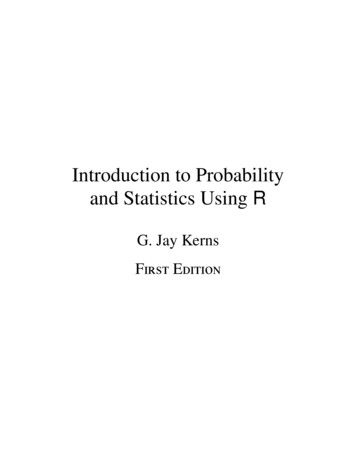
1.1.25aThe population of interest consists of voter opinions (for or against the candidate) at the time of theelection for all persons voting in the election.bNote that when a sample is taken (at some time prior or the election), we are not actually samplingfrom the population of interest. As time passes, voter opinions change. Hence, the population of voteropinions changes with time, and the sample may not be representative of the population of interest.1.1.26a-b The variable “survival time” is a quantitative continuous variable.cThe population of interest is the population of survival times for all patients having a particular typeof cancer and having undergone a particular type of radiotherapy.d-e Note that there is a problem with sampling in this situation. If we sample from all patients havingcancer and radiotherapy, some may still be living and their survival time will not be measurable. Hence,we cannot sample directly from the population of interest, but must arrive at some reasonable alternatepopulation from which to sample.1.1.27aThe variable “reading score” is a quantitative variable, which is probably integer-valued and hencediscrete.bThe individual on which the variable is measured is the student.cThe population is hypothetical – it does not exist in fact – but consists of the reading scores for allstudents who could possibly be taught by this method.Section 1.21.2.1The pie chart is constructed by partitioning the circle into five parts, according to the total contributed byeach part. Since the total number of students is 100, the total number receiving a final grade of Arepresents 31 100 0.31 or 31% of the total. Thus, this category will be represented by a sector angle of0.31(360) 111.6 . The other sector angles are shown next, along with the pie chart.Final GradeFrequencyFraction of TotalSector 310.8D9.0%F3.0%A31.0%C21.0%B36.0%2
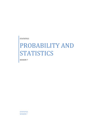
The bar chart represents each category as a bar with height equal to the frequency of occurrence of thatcategory and is shown in the figure that follows.40Frequency3020100ABCDFFinal Grade1.2.2Construct a statistical table to summarize the data. The pie and bar charts are shown in the figures thatfollow.StatusFrequencyFraction of TotalSector .1761.2Senior9.0932.4Grad Student8.0828.835Grad reJuniorSeniorGrad StudentStatusConstruct a statistical table to summarize the data. The pie and bar charts are shown in the figures thatfollow.StatusHumanities, Arts & SciencesNatural/Agricultural SciencesBusinessOtherFrequency43321783Fraction of Total.43.32.17.08Sector Angle154.8115.261.228.8
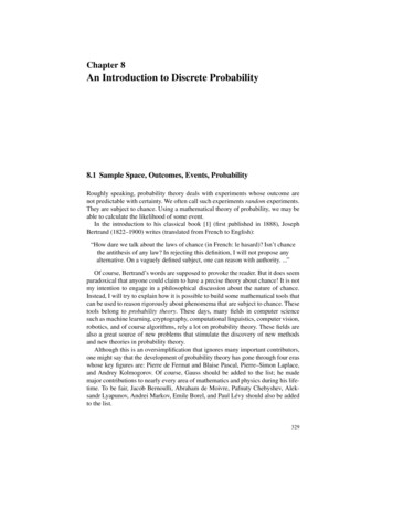
40Frequencyother8.0%Business17.0%Humanities, Arts & Sciences43.0%3020100Natural/Agricultural Sciences32.0%mHurt,Aesi tians&esncieScNesncc e pie chart is constructed by partitioning the circle into four parts, according to the total contributedby each part. Since the total number of people is 50, the total number in category A represents11 50 0.22 or 22% of the total. Thus, this category will be represented by a sector angle of0.22(360) 79.2o . The other sector angles are shown below. The pie chart is shown in the figure thatfollows.CategoryFrequencyFraction of TotalSector The bar chart represents each category as a bar with height equal to the frequency of occurrence ofthat category and is shown in the figure above.cYes, the shape will change depending on the order of presentation. The order is unimportant.dThe proportion of people in categories B, C, or D is found by summing the frequencies in those threecategories, and dividing by n 50. That is, (14 20 5) 50 0.78 .eSince there are 14 people in category B, there are 50 14 36 who are not, and the percentage iscalculated as ( 36 50 )100 72% .1.2.5a-b Construct a statistical table to summarize the data. The pie and bar charts are shown in the figuresthat follow.4
StateCAAZTXFrequency988Fraction of Total.36.32.32Sector 210AZ32.0%CAAZTXStatecFrom the table or the chart, Texas produced 8 25 0.32 of the jeans.dThe highest bar represents California, which produced the most pairs of jeans.eSince the bars and the sectors are almost equal in size, the three states produced roughly the samenumber of pairs of jeans.1.2.6-9 The bar charts represent each category as a bar with height equal to the frequency of occurrence of thatcategory.Exercise 7Exercise publicansIndependents0Democrats18 to 3435 to 5455 AgeParty IDExercise 8Exercise cansIndependents0Democrats18 to 3435 to 5455 AgeParty ID1.2.10Answers will vary.1.2.11aThe percentages given in the exercise only add to 94%. We should add another category called“Other”, which will account for the other 6% of the responses.bEither type of chart is appropriate. Since the data is already presented as percentages of the wholegroup, we choose to use a pie chart, shown in the figure that follows.5
Too much arguing5.0%other6.0%Not good at it14.0%Other plans40.0%Too much work15.0%Too much pressure20.0%c-d Answers will vary.1.2.12-14The percentages falling in each of the four categories in 2017 are shown next (in parentheses), and thepie chart for 2017 and bar charts for 2010 and 2017 follow.Region2010United States/Canada201799183 (13.8%)107271 (20.4%)Asia64453 (34.2%)Rest of the World58419 (31.6%)3281326 (100%)EuropeTotalExercise 12 (2017)U.S./Canada13.8%Rest of the World31.6%Europe20.4%Asia34.2%Exercise 14 (2017)Exercise 13 (2010)500100Average Daily Users (millions)Average Daily Users (millions)120806040200U.S./CanadaEuropeAsiaRest of the n6Rest of the World
1.2.15Users in Asia and the rest of the world have increased more rapidly than those in the U.S., Canada orEurope over the seven-year period.1.2.16aThe total percentage of responses given in the table is only (40 34 19)% 93% . Hence there are7% of the opinions not recorded, which should go into a category called “Other” or “More than a fewdays”.bYes. The bars are very close to the correct proportions.cSimilar to previous exercises. The pie chart is shown next. The bar chart is probably more interestingto look at.Mor than a Few Days7.0%No Time19.0%One Day40.0%A Few Days34.0%1.2.17-18 Answers will vary from student to student. Since the graph gives a range of values for Zimbabwe’s share,we have chosen to use the 13% figure, and have used 3% in the “Other” category. The pie chart and barcharts are shown next.other3.0%25Botswana26.0%20Percent 10.0%South Africa10.0%15BotswanaZimbabweAngolaSouth AfricaCanadaRussiaOtherCountry1.2.19-20 The Pareto chart is shown below. The Pareto chart is more effective than the bar chart or the pie chart.25Percent th AfricaOtherCountry1.2.21The data should be displayed with either a bar chart or a pie chart. The pie chart is shown next.7
lver13.9%White/White pearl20.8%Black/Black effect20.8%Red10.9%Gray16.8%Blue8.9%Section 1.31.3.1The dotplot is shown next; the data is skewed right, with one outlier, x 2.0.1.01.21.41.61.82.0Exercise 11.3.2The dotplot is shown next; the data is relatively mound-shaped, with no outliers.5456586062Exercise 21.3.3-5 The most obvious choice of a stem is to use the ones digit. The portion of the observation to the right ofthe ones digit constitutes the leaf. Observations are classified by row according to stem and also withineach stem according to relative magnitude. The stem and leaf display is shown next.1 6 82 1 2 5 5 5 7 8 8 9 93 1 1 4 5 5 6 6 6 7 7 7 7 8 9 9 9leaf digit 0.14 0 0 0 1 2 2 3 4 5 6 7 8 9 9 91 2 represents 1.25 1 1 6 6 76 123.The stem and leaf display has a mound shaped distribution, with no outliers.4.From the stem and leaf display, the smallest observation is 1.6 (1 6).5.The eight and ninth largest observations are both 4.9 (4 9).8
1.3.6The stem is chosen as the ones digit, and the portion of the observation to the right of the ones digit is theleaf.3 2 3 4 5 5 5 6 6 7 9 9 9 94 0 0 2 2 3 3 3 4 4 5 8leaf digit 0.1 1 2 represents 1.21.3.7-8 The stems are split, with the leaf digits 0 to 4 belonging to the first part of the stem and the leaf digits 5 to 9belonging to the second. The stem and leaf display shown below improves the presentation of the data.3 2 3 43 5 5 5 6 6 7 9 9 9 9leaf digit 0.1 1 2 represents 1.24 0 0 2 2 3 3 3 4 44 5 81.3.9The scale is drawn on the horizontal axis and the measurements are represented by dots.012Exercise 91.3.10Since there is only one digit in each measurement, the ones digit must be the stem, and the leaf will be azero digit for each measurement.0 0 0 0 0 01 0 0 0 0 0 0 0 0 02 0 0 0 0 0 01.3.11The distribution is relatively mound-shaped, with no outliers.1.3.12The two plots convey the same information if the stem and leaf plot is turned 90 o and stretched to resemblethe dotplot.1.3.13The line chart plots “day” on the horizontal axis and “time” on the vertical axis. The line chart shown nextreveals that learning is taking place, since the time decreases each successive day.45Time (seconds)4035302512345Day1.3.14The line graph is shown next. Notice the change in y as x increases. The measurements are decreasingover time.9
6362Measurement6160595857560246810Year1.3.15The dotplot is shown next.1234567Number of Cheeseburgers1.3.16aThe distribution is somewhat mound-shaped (as much as a small set can be); there are no outliers.b2 10 0.2aThe test scores are graphed using a stem and leaf plot generated by Minitab.b-c The distribution is not mound-shaped, but is rather has two peaks centered around the scores 65 and85. This might indicate that the students are divided into two groups – those who understand the materialand do well on exams, and those who do not have a thorough command of the material.1.3.17aWe choose a stem and leaf plot, using the ones and tenths place as the stem, and a zero digit as theleaf. The Minitab printout is shown next.10
Dotplot of CalciumbThe data set is relatively mound-shaped, centered at 5.2.cThe value x 5.7 does not fall within the range of the other cell counts, and would be consideredsomewhat unusual.1.3.18a-b The dotplot and the stem and leaf plot are drawn using e measurements all seem to be within the same range of variability. There do not appear to be anyoutliers.1.3.19a Stem and leaf displays may vary from student to student. The most obvious choice is to use the tensdigit as the stem and the ones digit as the leaf.7 8 98 0 1 79 0 1 2 4 4 5 6 6 6 8 810 1 7 911 2b The display is fairly mound-shaped, with a large peak in the middle.1.3.20aThe sizes and volumes of the food items do increase as the number of calories increase, but not in thecorrect proportion to the actual calories. The differences in calorie content are not accurately portrayed inthe graph.bThe bar graph which accurately portrays the number of calories in the six food items is shown next.11
900800Number of Calories7006005004003002001000Hershey's KissOreo12 oz Coke12 oz BeerPizzaWhopperFood Item1.3.21a-b The bar charts for the median weekly earnings and unemployment rates for eight different levels ofeducation are shown next.20008Median wkly earningsUnemployment steasgrdeeecBar' ucational AttainmentEducational amc The unemployment rate drops and the median weekly earnings rise as the level of educational attainmentincreases.1.3.22a Similar to previous exercises. The pie chart is shown next.Judaism0.2%Chinese mal Indigenous & African 15.6%bThe bar chart is shown next.12
Members (millions)2000150010005000hiddBusms tiriChiantynHiPrciduimsmdiInalIslusnoge&amf OterReligionThe Pareto chart is a bar chart with the heights of the bars ordered from large to small. This display is moreeffective than the pie chart.Members nundHimiss&ouendigAncafrialonit Religion1.3.23aThe distribution is skewed to the right, with a several unusually large measurements. The five statesmarked as HI are California, New Jersey, New York and Pennsylvania.bThree of the four states are quite large in area, which might explain the large number of hazardouswaste sites. However, New Jersey is relatively small, and other large states do not have unusually largenumber of waste sites. The pattern is not clear.1.3.24aThe distribution is skewed to the right, with two outliers.bThe dotplot is shown next. It conveys nearly the same information, but the stem-and-leaf plot may bemore informative.13
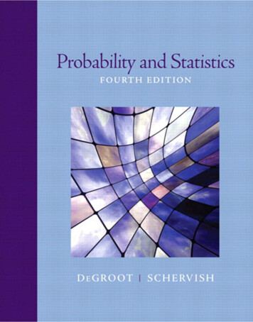
1.42.84.25.67.08.49.8Weekend Gross1.3.25aAnswers will vary.bThe stem and leaf plot is constructed using the tens place as the stem and the ones place as the leaf.Notice that the distribution is roughly mound-shaped.c-d Three of the five youngest presidents – Kennedy, Lincoln and Garfield – were assassinated while inoffice. This would explain the fact that their ages at death were in the lower tail of the distribution.Section 1.41.4.1The relative frequency histogram displays the relative frequency as the height of the bar over theappropriate class interval and is shown next. The distribution is relatively mound-shaped.50Relative ce the variable of interest can only take integer values, the classes can be chosen as the values 0, 1, 2, 3,4, 5 and 6. The table containing the classes, their corresponding frequencies and their relative frequenciesand the relative frequency histogram are shown next. The distribution is skewed to the right.14
Number of Household Pets0123456TotalFrequency131912410150Relative Frequency13/50 .2619/50 .3812/50 .244/50 .081/50 .020/50 .001/50 .0250/50 1.00.40Relative Frequency.30.20.1000123456Number of Pets1.4.3-8 The proportion of measurements falling in each interval is equal to the sum of the heights of the bars overthat interval. Remember that the lower class boundary is included, but not the upper class boundary.3. .20 .40 .15 .754. .05 .15 .20 .405. .056. .40 .15 .557. .158. .05 .15 .20 .401.4.9Answers will vary. The range of the data is 110 10 90 and we need to use seven classes. Calculate90 / 7 12.86 which we choose to round up to 15. Convenient class boundaries are created, starting at 10:10 to 25, 25 to 40, , 100 to 115.1.4.10Answers will vary. The range of the data is 76.8 25.5 51.3 and we need to use six classes. Calculate51.3 / 6 8.55 which we choose to round up to 9. Convenient class boundaries are created, starting at 25:25 to 34, 34 to 43, , 70 to 79.1.4.11Answers will vary. The range of the data is 1.73 .31 1.42 and we need to use ten classes. Calculate1.42 /10 .142 which we choose to round up to .15. Convenient class boundaries are created, starting at.30: .30 to .45, .45 to .60, , 1.65 to 1.80.1.4.12Answers will vary. The range of the data is 192 0 192 and we need to use eight classes. Calculate192 / 8 24 which we choose to round up to 25. Convenient class boundaries are created, starting at 0: 0to 25, 25 to 50, , 175 to 200.1.4.13-16 The table containing the classes, their corresponding frequencies and their relative frequencies and therelative frequency histogram are shown next.15
Class iClass BoundariesTallyfiRelative frequency, fi/n123451.6 to 2.12.1 to 2.62.6 to 3.13.1 to 3.63.6 to 4.11111111111111111111111 11111 1111255514.04.10.10.10.286789104.1 to 4.64.6 to 5.15.1 to 5.65.6 to 6.16.1 to 6.611111 1111111111111175232.14.10.04.06.04Relative .6DATA13. The distribution is roughly mound-shaped.14. The fraction less than 5.1 is that fraction lying in classes 1-7, or ( 2 5 15. The fraction larger than 3.6 lies in classes 5-10, or (14 7 7 5) 50 43 50 0.86 . 3 2 ) 50 33 50 0.66 .16. The fraction from 2.6 up to but not including 4.6 lies in classes 3-6, or( 5 5 14 7 ) 50 31 50 0.62 .1.4.17-20 Since the variable of interest can only take the values 0, 1, or 2, the classes can be chosen as the integervalues 0, 1, and 2. The table shows the classes, their corresponding frequencies and their relativefrequencies. The relative frequency histogram follows the table.Value012Frequency596Relative Frequency.25.45.3016
0.5Relative Frequency0.40.30.20.10.001217. Using the table above, the proportion of measurements greater than 1 is the same as the proportion of“2”s, or 0.30.18. The proportion of measurements less than 2 is the same as the proportion of “0”s and “1”s, or0.25 0.45 .70 .19. The probability of selecting a “2” in a random selection from these twenty measurements is 6 20 .30 .20. There are no outliers in this relatively symmetric, mound-shaped distribution.1.4.21-23 Answers will vary. The range of the data is 94 55 39 and we choose to use 5 classes. Calculate39 / 5 7.8 which we choose to round up to 10. Convenient class boundaries are created, starting at 50 andthe table and relative frequency histogram are created.Class Boundaries50 to 6060 to 7070 to 8080 to 9090 to 100Frequency26363Relative Frequency.10.30.15.30.15.30Relative Frequency.25.20.15.10.0505060708090100Scores21. The distribution has two peaks at about 65 and 85. Depending on the way in which the studentconstructs the histogram, these peaks may or may not be clearly seen.17
22. The shape is unusual. It might indicate that the students are divided into two groups – those whounderstand the material and do well on exams, and those who do not have a thorough command of thematerial.23. The shapes are roughly the same, but this may not be the case if the student constructs the histogramusing different class boundaries.1.4.24 aThere are a few extremely small numbers, indicating that the distribution is probably skewed to theleft.bThe range of the data 165 8 157 . We choose to use seven class intervals of length 25, withsubintervals 0 to 25, 25 to 50, 50 to 75, and so on. The tally and relative frequency histogram areshown next.Class i1234567Class Boundaries0 to 2525 to 5050 to 7575 to 100100 to 125125 to 150150 to 175Tally111111111111111 11111fi2033273Relative frequency, fi/n2/200/203/203/202/207/203/20.40Relative The distribution is indeed skewed left with two possible outliers: x 8 and x 11.aThe range of the data 32.3 0.2 32.1 . We choose to use eleven class intervals of length 3 (32.1 11 2.9 , which when rounded to the next largest integer is 3). The subintervals 0.1 to 3.1, 3.1 to 6.1, 6.1 to 9.1, and so on, are convenient and the tally and relative frequency histogram are shown next.Class i1234567891011Class Boundaries0.1 to 3.13.1 to 6.16.1 to 9.19.1 to 12.112.1 to 15.115.1 to 18.118.1 to 21.121.1 to 24.124.1 to 37.127.1 to 30.130.1 to 33.1Tally11111 11111 1111111111 111111111 11111111111111111111118fi1591034322101Relative frequency, fi/n15/509/5010/503/504/503/502/502/501/500/501/50
0.30Relative .1TIMEbThe data is skewed to the right, with a few unusually large measurements.cLooking at the data, we see that 36 patients had a disease recurrence within 10 months. Therefore, thefraction of recurrence times less than or equal to 10 is 36 50 0.72 .1.4.26aWe use class intervals of length 5, beginning with the subinterval 30 to 35. The tally and the relativefrequency histogram are shown next.Class i123456Class Boundaries30 to 3535 to 4040 to 4545 to 5050 to 5555 to 60Tally11111 11111 1111111 11111 1111111111 11111 1111111 111111fi121512821Relative frequency, fi/n12/5015/5012/508/502/501/50.30Relative Frequency.25.20.15.10.05030354045505560AgesbUse the table or the relative frequency histogram. The proportion of children in the interval 35 to 45is (15 12)/50 .54.c1.4.27The proportion of children aged less than 50 months is (12 15 12 8)/50 .94.aThe data ranges from .2 to 5.2, or 5.0 units. Since the number of class intervals should be betweenfive and twelve, we choose to use eleven class intervals, with each class interval having length 0.50 (5.0 11 .45 , which, rounded to the nearest convenient fraction, is .50). We must now select i
2 1.1.25 a The population of interest consists of voter opinions (for or against the candidate) at the time of the election for all persons voting in the election. b Note that when a sample is taken (at some time prior or the election), we are not actually sampling from the population of interest. As time passes, voter opinions change. Hence, the population of voter