WIXLIB

2LINEAR ALGEBRA, ilizer LevelFIGURE 1.1 Regression of yield on fertilizer level.C and D.This model may not be a good approximation of the true regression function,and, if possible, should be checked for validity. The crop yield as a function offertilizer level may well have the form in Figure 1.1.The regression function g would be better approximated by a second degreepolynomial y(x) A Bx Cx2. However, if attention is confined to the 0.7to 1.3 range, the regrcssion function is approximately linear, and the simplifyingmodel y(x) C D.u, called the simple linear regression model, may be used.In attempting to understand the relationship between a person's height Yand the heights of hisiher father (xl) and mother (xZ) and the person's sex (xJ.we might supposeg(x) then becomes the simpler one of estimating the two parameterswhere .x3 is 1 for males, 0 for females, and Po, PI. p2, ps are unknownparameters. Thus a brother would be expected to be P3 taller than his sister.Again, this model, called a multiple regression model, can only be an approximation of the true regression function, valid over a limited range of values ofx l , x2. A more complex model might suppose

3VECTORS, lNNER PRODUCTS, LENGTHSTable 1.1.1Indiv.12345678910Height 0This model is nonlinear in (xl, x2, x3), but linear in the Fs. It is the linearityin the p's which makes this model a linear statistical model.Consider the model ( l . l . l ) , and suppose we have data of Table 1.1.1 on( Y , x , , x z , x 3 ) for 10 individuals. These data were collected in a class taughtby the author. Perhaps the student can collect similar data in his or her classand compare results.b,, &, b, so that theThe statistical problem is to determine estimatesresulting function d(x,, x2, x3) B,x, B2x2 B,x3 is in some sense agood approximation of g(x,, x2, x3). For this purpose it is convenient to writethe model in vector form:Po b0, where xo is the vector of all ones, and y and xlr x2, x3 are the column vectorsin Table 1.1.1.This formulation of the model suggests that linear algebra may be animportant tool in the analysis of linear statistical models. We will thereforereview such material in the next section, emphasizing geometric aspects.1.2 VECTORS, INNER PRODUCI'S, LENGTHSLet R be the collection of all n-tuples of real numbers for a positive integer n.In applications R will be the sample space of all possible values of theobservation vector y. Though 2 will be in one-to-one correspondence toEuclidean n-space, it will be convenient to consider elements of Q as arrays allof the same configuration, not necessarily column or row vectors. For example,in application to what is usually called one-way analysis of variance, we might

4LINEAR ALGEBRA. PROJECTIONShave 3,4 and 2 observations on three different levels of some treatment effect.Then we might takeYlZYzzY32)14 Zand 0 the collection of all such y- While we could easily reform y into a columnvector, it is often convenient to preserve the form of y. The term "n-tuple"means that the elements of a vector y f R are ordered. A vector y may beconsidered to be a real-valued function on { 1,. . .,n } .R becomes a linear space if we define ay for any y E R and any real numbera to be the element of R given by multiplying each component of R by a, andif for any two elements yl, yz E R we define yl yz to be the vector in R whoseith component is the sum of the ith components of y, and y2, for i 1, . . . , n.R becomes an inner product space if for each x, y E R we define the functionwhere x ( x l , . . , x n ) and y { y , , . . . , y . ) . If R is the collection of ndimensional column vectors then h(x, y) x'y, in matrix notation. The innerproduct h(x, y) is usually written simply as (x, y), and we will use this notation.The inner product is often called the dot product, written in the form x - y . Sincethere is a small danger of confusion with the pair (x, y), we will use boldparentheses to emphasize that we mean the inner product. Since bold symbolsare not easily indicated on a chalkboard or in student notes, it is importantthat the meaning will almost always be clear from the context. The innerproduct has the properties:for all vectors, and real numbers a.We define \lx\\' (x, x) and call llxll the {Euclidean) length of x. Thusx (3,4, 12) has length 13.The distance between vectors x and y is the length of x - y. Vectors x andy are said to be orthogonal if (x, y) 0. We write x Iy.

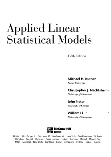
5VECTORS, MNER PRODUCTS, LENGTHSFor example, if the sample space is the collection of arrays mentioned above,thenare orthogonal, with squared lengths 14 and 36. For R the collection of 3-tuples,(2,3, 1) I (- I , 1, - 1).The following theorem is perhaps the most important of the entire book.We credit it to Pythagorus (sixth century B.c.), though he would not, of course,have recognized it in this form.Pythagorean Tbeorem: Let v,, . . . ,vk be mutually orthogonal vectors in RThenDebition 1.21:such thatThe projection of a vector y on a vector x is the vector 91. 9 bx for some constant b2. (y - 5) I x (equivalently, (9, x) (y, x))Equivalently, 3 is the projection of y on the subspace of all vectors of the formax, the subspace spanned by x (Figure 1.2). To be more precise, these propertiesdefine othogonal projection. We will use the word projection to mean orthogonal projection. We write p(ylx) to denote this projection. Students shouldnot confuse this will conditional probability.Let us try to find the constant b. We need (9, x) (bx, x) b(x, x) (y, x).Hence, if x 0, any b will do. Otherwise, b (y, x)/[lxl12. Thus,[(y,X)/IIXI( ]X,for x 0otherwiseHere 0 is the vector of all zeros. Note that if x is replaced by a multiple ax ofx, for a # 0 then 9 remains the same though the coefficient 6 is replaced by 6/a

6LINEAR ALGEBRA, PROJECTIONSAYXFIGURE 1.2Theorem 1.2.1: Among all multiples ux of x, the projectionthe closest vector to y.9 of y on xisProof: Since (y - 9) I ( 9 - ax) and (y - ax) (y - 9 ) (9 - ax), itfollows that11y- ax112 !(y - 11’This is obviously minimum for ux 9. iI - uxI12.I1Since 3 I (y - 9) and y 9 (y - 9), the Pythagorean Theorem implies, impliesthat IIyilz 11911’ I/y - 9112. Since [19iI2 b211xIIZ (y, X ) / I I X I I this\ , equality if and only if Ily - 911 0, i.e., y is athat !Iyilz 2 (y, ) / l l x lwithmultiple of x. This is the famous Cauchy-Schwurz Inequality, usually writtenas (y, x ) Illy112/1x112.The inequality is best understood as the result of theequality implied by the Pythagorean Theorem.Definition 1.2.2: Let A be a subset of the indices of the components of avector space R. The indicator of A is the vector I, E !2, with components whichare 1 for indices in A, and 0 otherwise.The projection 9, of y on the vector I, is therefore hl, for b (y. I , ) / l l k 2(2y[)/N(A),where N ( A ) is the number of indices in A. Thus, h j A , the

7SUBSPACES, PROJECTIONSmean of the y-values with components in A. For example, if R is the space of4-component row vectors, y (3,7,8,13), and A is the indicator of the secondand fourth components, p(yl1,) (0,10, 0,lO).)Problem 1.2.1: Let R be the collection of all 5-tuples of the formy (‘”).Letx (”211 0).y (’2 1 39 4 11(a) Find (x, y), I I X Ilyl12, , 9 p(yIx), and y - 9. Show that x I(y - j ) , andYlZIIYII’ Y22y.31119112 IIY - 911’.(-21)and z 3x 2n. Show that (w, x) 0 and that0 2 01!z)1’ 911x)j’ 4[1wl12.(Why must this be true?)(c) Let x,, x‘, x3 be the indicators of the first, second and third columns.Find p(y)x,) for i 1, 2, 3.(b) Let w Problem 12.2: Is projection a linear transformation in the sense thatp(cyIx) cp(ylx) for any real number c? Prove or disprove. What is therelationship between p(y(x) and p(yicx) for c # O?Problem 1.23: Let l1x11’ 0. Use calculus to prove that I/y - hxII’ isminimiim for b (y, x)/IIxlI’.IIxProblem 134: Prove the converse of the Pythagorean Theorem. That is, yi12 llxll’ illyll’ implies that x 1y.Problem 1.2.5:1.3Sketch a picture and provc the parallelogram law:SUBSPACES, PROJECTIONSWe begin the discussion of subspaces and projections with a number ofdefinitions of great importance to our subsequent discussion of linear models.Almost all of the definitions and the theorems which follow are usually includedin a first course in matrix or linear algebra. Such courses do not always includediscussion of orthogonal projection, so this material may be new to the student.Defioition 1.3.1: A subspuce of R is a subset of R which is closed underaddition and scalar multiplication.That is, V c R is a subspace if for every x E V and every scalar a, ax E Vand if for every vl, v2 E V, vI v2 E V.

8LINEAR ALGEBRA. PROJECTIONSDefinition 1.3.2: Let xl,. . . ,x k be k vectors in an n-dimensional vectorspace. The subspace spanned by x , , . . . ,x k is the collection of all vectorsfor all real numbers b,, . . . ,bk. We denote this subspace by Y ( x , , . . . , x k ) .Definition 133: Vectors x , , . . . ,x k are linearly independent ifimplies b, 0 for i 1,. . . ,k.t1bixi OIDefinition 13.4: A busis for a subspace V of f2 is a set of linearlyindependent vectors which span V .The proofs of Theorems 1.3.1 and 1.3.2 are omitted. Readers are referred toany introductory book on linear algebra.Tbeorem 1.3.1: Every basis for a subspace V on 2 has the same numberof elements.Definition 13.5: The dimension of a subspace Y of Q is the number ofelements in each basis.Theorem 13.2: Let v,, . . . ,vk be linearly independent vectors in a subspaceV of dimension J . Then d 2 k.Comment: Theorem 1.3.2 implies that if dim( V) d then any collection ofd 1 or more vectors in V must be linearly dependent. In particular, anycollection of n 1 vectors in the n-component space R are linearly dependent.Definition 13.6: A vector y is orthogonal to a subspace V of Q if y isorthogonal to all vectors in V. We write y L V.Problem 1.3.1: Let Q be the space of all 4component row vectors.Let x 1 ( 1, 1, 1, 1), X I ; (1, 1,0, O), 3 (1,0, 1,0), 4 (7,4,9,6). Let Vz V ( x 1 ,X A Vs Y(x,, 2 x j, ) and V, Y ( x 1 , 2 r 3 9 4 ) .(a) Find the dimensions of Vz and V,.which contain vectors with as many zeros as(b) Find bases for V2 andpossible.(c) Give a vector z # 0 which is orthogonal to all vectors in V,.(d) Since x l , x2, xg, z are linearly independent, x4 is expressible in the form31b,xi cz. Show that c 0 and hence that x4 E V,, by determining ( x 4 ,2).What is dim( V,)?(e) Give a simple verbal description of V3.

[:::SUBSPACES. PROJECTIONS9Y2,Problem 13.2: Consider the space R of arrays y , 2 y,,and defineC,,C2.C3to be the indicators of the columns. Let V Y ( C , ,Cz,C3).(a) What properties must y satisfy in order that y E M In order that y IM(b) Find a vector y which is orthogonal to V.The following definition is perhaps the most important in the entire book.It serves as the foundation of all the least squares theory to be discussed inChapters 1, 2, and 3.Definition 1.3.7: The projection of a vector y on a subspace Y of R is thevector 9 E V such that (y - 9) I V. The vector y - 9 e will be called theresidual vector for y relative to V.Comment: The condition (y - 9 ) 1 V is equivalent to (y - f, x) 0 for allx E V . Therefore, in seeking the projection f of y on a subspace V we seek avector 9 in V which has the same inner products as y with all vectors in V(Figure 1.3).If vectors x,. . . . ,x k span a subspace V then a vector z E V is the projectionckof y on V if (z, x i ) (y. x i ) for all i, since for any vector x implies thatj-bjxlEV, this1It is tempting to attempt to compute the projection f of y on V by simplysumming the projections f i p(yIx,). As we shall see, this is only possible insome very special cases.FIGURE 13

10LINEAR ALGEBRA, PROJECTIONSAt this point we have not established the legitimacy of Definition 1.3.7. Doessuch a vector 9 always exist and, if so, is it unique? We do know that theprojection onto a one-dimensional subspace, say onto V 9(x), for x # 0,does exist and is unique. In factExample 13.1:Consider the 6-component space Q of the problem above,i6and let V 2(Cl,C2,C3). Let y 10 8\ s7\. It is easy to show that theJvector 9 Ep(yJC,) 7C1 6C2 7C3 satisfies the conditions for a projection onto V. As will soon be shown the representation of f as the sum ofprojections on linearly independent vectors spanning the space is possiblebecause C,,C,, and C3 are mutually othogonal.We will first show uniqueness of the projection. Existence is more difficult.Suppose 9 , and g2 are two such projections of y onto V. Then f 1- 9, E V and(9, - 9,) (y - 9,) - (y - fl)is orthogonal to all vectors in V , in particularto itself. Thus llf, - 9,112 (PI - y,, 9, - jl,) 0, implying - f2 0, i.e.,9, 92.We have yet to show that 4 always exists. In the case that it does exist (wewill show that it always exists) we will write 9 p(yl Vj.If we are fortunate enough to have an orthogonal basis (a basis of mutuallyorthogonal vectors) for a given subspace V, it is easy to find the projection.Students are warned that that method applies only for an orthogonal basis. Wewill later show that all subspaces possess such orthogonal bases, so that theprojection 9 p(yl V) always exists.Theorem 133: Let v,, . . . ,vk be an orthogonal basis for V, subspace of R.ThenPOIkv) iCP(YIvi) 1Proof: Let fi p(ylv,) hivi for hi (y, vi)/Ilvi112. Since 3,- is a scalarmultiple of vi, it is orthogonal to vj forj # i.From the comment on the previousand y, have the same inner product withpage, we need only show thateach vj, since this implies that they have the same inner product with all x E V.Butcfi

11SUBSPACES, PROJECTIONSExample 13.2:LetThen v1 I v2 andThen (y, v l ) 9, (y, v2) 12, (9, vl) 9, and (9, v,) 12. The residual vector isy-9 /-o\which is orthogonal to V.Would this same procedure have worked if we replaced this orthogonal basisv!, v1 for Y by a nonorthogonal basis? To experiment, let us leave v, in thenew basis, but replace v2 by v3 2v, - v2. Note that lip(vl, v3) 9 ( v I , v2) V,and that (v,, v2) # 0. f I remains the same. v3 2v, - v2 , which has inner products 11 and 24 with v1 and v3.is not orthogonal to V. Therefore, 9, j 3 is not theprojection of y on V Y ( v l , v3).Since (y - 9) I 9, we have, by the Pythagorean Theorem,l!Y!I2 IKY - 9 ) HI2 IlY - 9112 1191r’llyllz 53,11f112 92123 6 51,IIy- j1I2 I(-‘)i2 2.1Warning: We have shown that when v l , . .,vk are mutually orthogonal

12LINEAR ALGEBRA, PROJECTIONSthe projection 3 of y on the subspace spanned by vl, . . . ,vk isk/ 1p(y(vj). Thisis true for all y only if vI, . . . ,vk are mutually orthogonal. Students are askedto prove the “only” part in Problem 1.3.5.Every subspace V of R of dimension r 0 has an orthogonal basis (actuallyan infinity of such bases). We will show that such a basis exists by usingGram-Schmidt orthogonalization.Let xl,. . . ,xk be a basis for a subspace V, a kdimensional subspace of Q.For 1 5 i 5 k let 6 U(xl, . . . ,xi) so that V, c 6 t * * c 5 are properlynested subspaces. Letv1 Xl,v2 x2- p(X,lV,). Then vl and v2 span 6 and are othogonal. Thus p(x3( V,) p(x,lv,)p(x31v2)and we can define v3 x3 - p(x3JVz).Continuing in this way, suppose we havedefined vl, ., vi to be mutually orthogonal vectors spanning 6. Definevi l xi , - ( X Jo. ThenIvi l 1 and hence v,, . .,vi I are mutuallyorthogonal and span c l. Since we can do this for each i Ik - 1 we get theorthogonal basis vl,. . . ,vk for V.If {vl,. . . ,v k } is an orthogonal basis for a subspace V then, since f 2 p(ylv,)kP(yl V ) j- 1and p(ylvj) bjvj, with b, [(y, v,)/IIvjl12],it follows bythe Pythagorean Theorem thatkkkOf course, the basis {vl,. . . ,vk) can be made into an orthonormal basis (allvectors of length one) by dividing each by its own length. If {v:, . . . ,v:) is suchan orthonormal basis thencki 13 p(yl V ) kk1p(ylv’) C (y. vf)vf1and11911’ (YN2.[ \ ,: ’ ],E x a m p l e 1.3.3: Consider R,, the space of Ccomponent column vectors.Let us apply Gram--Schmidt orthogonalization to the columns of X a matrix chosen carefully by the author to keep the5810

13SUBSPACES, PROJECTIONSarithmetic simple. Let the four columns be xlr. , x4. Define v 1 xl. Let,v 3 x 3 - [ r * , * 6 v322 ] -22L -2.andWe can multiply these vI by arbitrary constants to simplify them without losingtheir orthogonality. For example, we can define ui vi/l vil12, so that u,, u2,u3, u, are unit length orthogonal vectors spanning R. Then U (ul, u2, u3,u4)is an orthogonal matrix. U is expressible in the form U XR, where R haszeros below the diagonal. Since I U'U U'XR, R - U'X, and X UR- ',where R-' has zeros below the diagonal (see Section 1.7).'As we consider linear models we will often begin with a model whichsupposes that Y has expectation 8 which lies in a subspace b,and will wishto decide whether this vector lies in a smaller subspace V,. The orthogonalbases provided by the following theorem will be useful in the development ofconvenient formulas and in the investigation of the distributional properties ofestimators.Theorem 1.3.4: Let V, c V, c R be subspaces of Q of dimensions1 5 n, c n, c n. Then there exist mutually orthogonal vectors vl, . . . ,v, suchthat vI,. . . , v,, span F, i 1, 2.Proof: Let {xl,. .,x,,} be a basis for V,. Then by Gram-Schmidtorthogonalization there exists an orthogonal basis (vl,. . . ,v,,} for V,. Letx,, l , . . . ,xnZbe chosen consecutively from V2 so that vI, . . . ,v,,,, x,,, . . ,

Stapleton, James, 1931- Linear statistical models 1 James Stapleton. p. cm. Wiley series in probability and statistics. Probability and statistics section) "A Wilcy-Interscience publication." ISBN -471-57150-4 (acid-free) 1. Linear models (Statistics) 1. Title. 11. Series. Ill. Series: Wiley series in probability and statistics.