Transcription
PROBABILITY AND STATISTICSMANJUNATH KRISHNAPURC ONTENTS1.What is statistics and what is probability?52.Discrete probability spaces73.Examples of discrete probability spaces124.Countable and uncountable175.On infinite sums196.Basic rules of probability237.Inclusion-exclusion formula258.Bonferroni’s inequalities289.Independence - a first look3010.Conditional probability and independence3111.Independence of three or more events3412.Discrete probability distributions3513.General probability distributions3814.Uncountable probability spaces - conceptual difficulties3915.Examples of continuous distributions4216.Simulation4717.Joint distributions5118.Change of variable formula5419.Independence and conditioning of random variables5820.Mean and Variance6221.Makov’s and Chebyshev’s inequalities6722.Weak law of large numbers6823.Monte-Carlo integration6924.Central limit theorem7025.Poisson limit for rare events7326.Entropy, Gibbs distribution741.Introduction772.Estimation problems783.Properties of estimates824.Confidence intervals851
5.Confidence interval for the mean896.Actual confidence by simulation907.Testing problems - first example928.Testing for the mean of a normal population949.Testing for the difference between means of two normal populations9510.Testing for the mean in absence of normality9711.Chi-squared test for goodness of fit9812.Tests for independence10013.Regression and Linear regression102Appendix A.Lecture by lecture plan110Appendix B.Various pieces1112
Probability4
1. W HAT IS STATISTICS AND WHAT IS PROBABILITY ?Sometimes statistics is described as the art or science of decision making in the face of uncertainty.Here are some examples to illustrate what it means.Example 1. Recall the apocryphal story of two women who go to King Solomon with a child, eachclaiming that it is her own daughter. The solution according to the story uses human psychologyand is not relevant to recall here. But is this a reasonable question that the king can decide?Daughters resemble mothers to varying degrees, and one cannot be absolutely sure of guessingcorrectly. On the other hand, by comparing various features of the child with those of the twowomen, there is certainly a decent chance to guess correctly.If we could always get the right answer, or if we could never get it right, the question would nothave been interesting. However, here we have uncertainty, but there is a decent chance of gettingthe right answer. That makes it interesting - for example, we can have a debate between eyeistsand nosists as to whether it is better to compare the eyes or the noses in arriving at a decision.Example 2. The IISc cricket team meets the Basavanagudi cricket club for a match. Unfortunately,the Basavanagudi team forgot to bring a coin to toss. The IISc captain helpfully offers his coin, butcan he be trusted? What if he spent the previous night doctoring the coin so that it falls on oneside with probability 3/4 (or some other number)?Instead of cricket, they could spend their time on the more interesting question of checking ifthe coin is fair or biased. Here is one way. If the coin is fair, in a large number of tosses, commonsense suggests that we should get about equal number of heads and tails. So they toss the coin100 times. If the number of heads is exactly 50, perhaps they will agree that it is fair. If the numberof heads is 90, perhaps they will agree that it is biased. What if the number of heads is 60? Or 35?Where and on what basis to draw the line between fair and biased? Again we are faced with thequestion of making decision in the face of uncertainty.Example 3. A psychic claims to have divine visions unavailable to most of us. You are assignedthe task of testing her claims. You take a standard deck of cards, shuffle it well and keep it facedown on the table. The psychic writes down the list of cards in some order - whatever her visiontells her about how the deck is ordered. Then you count the number of correct guesses. If thenumber is 1 or 2, perhaps you can dismiss her claims. If it is 45, perhaps you ought to be take herseriously. Again, where to draw the line?The logic is this. Roughly one may say that surprise is just the name for our reaction to an eventthat we á priori thought had low probability. Thus, we approach the experiment with the belief thatthe psychic is just guessing at random, and if the results are such that under that random-guesshypothesis they have very small probability, then we are willing to discard our preconception andaccept that she is a psychic.How low a probability is surprising? In the context of psychics, let us say, 1/10000. Once we fixthat, we must find a number m 52 such that by pure guessing, the probability to get more than5
m correct guesses is less that 1/10000. Then we tell the psychic that if she gets more than m correctguesses, we accept her claim, and otherwise, reject her claim. This raises the simple (and you cando it yourself)Question 4. For a deck of 52 cards, find the number m such thatP(by random guessing we get more than m correct guesses) 1.10000Summary: There are many situations in real life where one is required to make decisions underuncertainty. A general template for the answer could be to fix a small number that we allowas the probability of error, and deduce thresholds based on it. This brings us to the question ofcomputing probabilities in various situations.Probability: Probability theory is a branch of pure mathematics, and forms the theoretical basisof statistics. In itself, probability theory has some basic objects and their relations (like real numbers, addition etc for analysis) and it makes no pretense of saying anything about the real world.Axioms are given and theorems are then deduced about these objects, just as in any other part ofmathematics.But a very important aspect of probability is that it is applicable. In other words, there are manysituations in which it is reasonable to take a model in probabilityIn the example above, to compute the probability one must make the assumption that the deckof cards was completely shuffled. In other words, all possible 52! orders of the 52 cards areassumed to be equally likely. Whether this assumption is reasonable or not depends on how wellthe card was shuffled, whether the psychic was able to get a peek at the cards, whether someinsider is informing the psychic of the cards etc. All these are non-mathematical questions, andmust be decided on other basis.However.: Probability and statistics are very relevant in many situations that do not involve anyuncertainty on the face of it. Here are some examples.Example 5. Compression of data. Large files in a computer can be compressed to a .zip formatand uncompressed when necessary. How is it possible to compress data like this? To give a verysimple analogy, consider a long English word like invertebrate. If we take a novel and replace everyoccurrence of this word with “zqz”, then it is certainly possible to recover the original novel (since“zqz” does not occur anywhere else). But the reduction in size by replacing the 12-letter wordby the 3-letter word is not much, since the word invertebrate does not occur often. Instead, if wereplace the 4-letter word “then” by “zqz”, then the total reduction obtained may be much higher,as the word “then” occurs quite often.This suggests the following optimal way to represent words in English. The 26 most frequentwords will be represented by single letters. The next 26 26 most frequent words will be represented by two letter words, the next 26 26 26 most frequent words by three-letter words, etc.6
Assuming there are no errors in transcription, this is a good way to reduce the size of any textdocument! Now, this involves knowing what the frequencies of occurrences of various words inactual texts are. Such statistics of usage of words are therefore clearly relevant (and they could bedifferent for biology textbooks as compared to 19th century novels).Example 6. Search algorithms such as Google, use many randomized procedures. This cannotbe explained right now, but let us give a simple reason to say why introducing randomness is agood idea in many situations. In the game of rock-paper-scissors, two people simultaneously shoutone of the three words, rock, paper or scissors. The rule is that scissors beats paper, paper beatsrock and rock beats scissors (if they both call the same word, they must repeat). In a game likethis, although there is complete symmetry in the three items, it would be silly to have a fixedstrategy. In other words, if you decide to always say rock, thinking that it doesn’t matter whichyou choose, then your opponent can use that knowledge to always choose paper and thus win!In many games where the opponent gets to know your strategy (but not your move), the beststrategy would involve randomly choosing your move.2. D ISCRETE PROBABILITY SPACESDefinition 7. Let Ω be a finite or countable1 set. Let p : Ω [0, 1] be a function such thatPω Ω pω 1. Then (Ω, p) is called a discrete probability space. Ω is called the sample space andpω are called elementary probabilities. Any subset A Ω is called an event. For an event A we define its probability as P(A) Pω A pω . Any function X : Ω R is called a random variable. For a random variable we define itsPexpected value or mean as E[X] ω Ω X(ω)pω .All of probability in one line: Take an (interesting) probability space (Ω, p) and an (interesting)event A Ω. Find P(A).This is the mathematical side of the picture. It is easy to make up any number of probabilityspaces - simply take a finite set and assign non-negative numbers to each element of the set so thatthe total is 1.Example 8. Ω {0, 1} and p0 p1 21 . There are only four events here, , {0}, {1} and {0, 1}.Their probabilities are, 0, 1/2, 1/2 and 1, respectively.Example 9. Ω {0, 1}. Fix a number 0 p 1 and let p1 p and p0 1 p. The sample space isthe same as before, but the probability space is different for each value of p. Again there are onlyfour events, and their probabilities are P{ } 0, P{0} 1 p, P{1} p and P{0, 1} 1.1For those unfamiliar with countable sets, it will be explained in some detail later.7
Example 10. Fix a positive integer n. LetΩ {0, 1}n {ω : ω (ω1 , . . . , ωn ) with ωi 0 or 1 for each i n}.Let pω 2 n for each ω Ω. Since Ω has 2n elements, it follows that this is a valid assignment ofelementary probabilities.nThere are 2#Ω 22 events. One example is Ak {ω : ω Ω and ω1 . . . ωn k} where k issome fixed integer. In words, Ak consists of those n-tuples of zeros and ones that have a total of k many ones. Since there are nk ways to choose where to place these ones, we see that #Ak nk .Consequently, n 2 n#AkkP{Ak } pω n 02ω AkXab It will be convenient to adopt the notation thatif b 0. Then we can simply write P{Ak } nkif 0 k n,otherwise. 0 if a, b are positive integers and if b a or2 n without having to split the values of k intocases.Example 11. Fix two positive integers r and m. LetΩ {ω : ω (ω1 , . . . , ωr ) with 1 ωi m for each i r}.The cardinality of Ω is mr (since each co-ordinate ωi can take one of m values). Hence, if we setpω m r for each ω Ω, we get a valid probability space.rOf course, there are 2m many events, which is quite large even for small numbers like m 3and r 4. Some interesting events are A {ω : ωr 1}, B {ω : ωi 6 1 for all i}, C {ω : ωi 6 ωj if i 6 j}. The reason why these are interesting will be explained later. Because ofequal elementary probabilities, the probability of an event S is just #S/mr . Counting A: We have m choices for each of ω1 , . . . , ωr 1 . There is only one choice for ωr .Hence #A mr 1 . Thus, P(A) mr 1mr 1m. Counting B: We have m 1 choices for each ωi (since ωi cannot be 1). Hence #B (m 1)rand thus P(B) (m 1)rmr (1 1 rm) . Counting C: We must choose a distinct value for each ω1 , . . . , ωr . This is impossible ifm r. If m r, then ω1 can be chosen as any of m values. After ω1 is chosen, there are(m 1) possible values for ω2 , and then (m 2) values for ω3 etc., all the way till ωr whichhas (m r 1) choices. Thus, #C m(m 1) . . . (m r 1). Note that we get the sameanswer if we choose ωi in a different order (it would be strange if we did not!).Thus, P(C) m(m 1).(m r 1).mrNote that this formula is also valid for m r since oneof the factors on the right side is zero.8
2.1. Probability in the real world. In real life, there are often situations where there are severalpossible outcomes but which one will occur is unpredictable in some way. For example, when wetoss a coin, we may get heads or tails. In such cases we use words such as probability or chance,event or happening, randomness etc. What is the relationship between the intuitive and mathematicalmeanings of words such as probability or chance?In a given physical situation, we choose one out of all possible probability spaces that we thinkcaptures best the chance happenings in the situation. The chosen probability space is then called amodel or a probability model for the given situation. Once the model has been chosen, calculation ofprobabilities of events therein is a mathematical problem. Whether the model really captures thegiven situation, or whether the model is inadequate and over-simplified is a non-mathematicalquestion. Nevertheless that is an important question, and can be answered by observing the reallife situation and comparing the outcomes with predictions made using the model2.Now we describe several “random experiments” (a non-mathematical term to indicate a “reallife” phenomenon that is supposed to involve chance happenings) in which the previously givenexamples of probability spaces arise. Describing the probability space is the first step in any probability problem.Example 12. Physical situation: Toss a coin. Randomness enters because we believe that the coinmay turn up head or tail and that it is inherently unpredictable.The corresponding probability model: Since there are two outcomes, the sample space Ω {0, 1}(where we use 1 for heads and 2 for tails) is a clear choice. What about elementary probabilities?Under the equal chance hypothesis, we may take p0 p1 12 . Then we have a probability modelfor the coin toss.If the coin was not fair, we would change the model by keeping Ω {0, 1} as before but lettingp1 p and p0 1 p where the parameter p [0, 1] is fixed.Which model is correct? If the coin looks very symmetrical, then the two sides are equally likelyto turn up, so the first model where p1 p0 12is reasonable. However, if the coin looks irregular,then theoretical considerations are usually inadequate to arrive at the value of p. Experimentingwith the coin (by tossing it a large number of times) is the only way.There is always an approximation in going from the real-world to a mathematical model. Forexample, the model above ignores the possibility that the coin can land on its side. If the coin isvery thick, then it might be closer to a cylinder which can land in three ways and then we wouldhave to modify the model.2Roughly speaking we may divide the course into two parts according to these two issues. In the probability partof the course, we shall take many such models for granted and learn how to calculate or approximately calculateprobabilities. In the statistics part of the course we shall see some methods by which we can arrive at such models, ortest the validity of a proposed model.9
Thus we see that example 9 is a good model for a physical coin toss. What physical situationsare captured by the probability spaces in example 10 and example 11?Example 10: This probability space can be a model for tossing n fair coins. It is clear in what sense,so we omit details for you to fill in.The same probability space can also be a model for the tossing of the same coin n times insuccession. In this, we are implicitly assuming that the coin forgets the outcomes on the previoustosses. While that may seem obvious, it would be violated if our “coin” was a hollow lens filledwith a semi-solid material like glue (then, depending on which way the coin fell on the first toss,the glue would settle more on the lower side and consequently the coin would be more likely tofall the same way again). This is a coin with memory!Example 11: There are several situations that can be captured by this probability space. We listsome. There are r labelled balls and m labelled bins. One by one, we put the balls into bins “atrandom”. Then, by letting ωi be the bin-number into which the ith ball goes, we can capturethe full configuration by the vector ω (ω1 , . . . , ωn ). If each ball is placed completely atrandom then the probabilities are m r for each configuration ω.In that example, A is the event that the last ball ends up in the first bin, B is the eventthat the first bin is empty and C is the event that no bin contains more than one ball. If m 6, then this may also be the model for throwing a fair die r times. Then ωi is the outcome on the ith throw. Of course, it also models throwing r different (and distinguishable)fair dice. If m 2 and r n, this is same as Example 10, and thus models the tossing of n fair coins(or a fair coin n times). Let m 365. Omitting the possibility of leap years, this is a model for choosing r peopleat random and noting their birthdays (which can be in any of 365 “bins”). If we assumethat all days are equally likely as a birthday (is this really true?), then the same probabilityspace is a model for this physical situation. In this example, C is the event that no twopeople have the same birthday.The next example is more involved and interesting.Example 13. Real-life situation: Imagine a man-woman pair. Their first child is random, forexample, the sex of the child, or the height to which the child will ultimately grow, etc cannot bepredicted with certainty. How to make a probability model that captures the situation?10
A possible probability model: Let there be n genes in each human, and each of the genes can taketwo possible values (Mendel’s “factors”), which we denote as 0 or 1. Then, let Ω {0, 1}n {x (x1 , . . . , xn ) : xi 0 or 1}. In this sense, each human being can be encoded as a vector in {0, 1}n .To assign probabilities, one must know the parents. Let the two parents have gene sequencesa (a1 , . . . , an ) and (b1 , . . . , bn ). Then the possible offsprings gene sequences are in the set Ω0 : {x {0, 1}n : xi ai or bi , for each i n}. Let L : #{i : ai 6 bi }.One possible assignment of probabilities is that each of these offsprings is equally likely. In thatcase we can capture the situation in the following probability models.(1) Let Ω0 be the sample space and let px 2 L for each x Ω0 .(2) Let Ω be the sample space and let 2 Lpx 0if x Ω0if x 6 Ω0 .The second one has the advantage that if we change the parent pair, we don’t have to change thesample space, only the elementary probabilities. What are some interesting events? Hypothetically, the susceptibility to a disease X could be determined by the first ten genes, say the person islikely to get the disease if there are at-most four 1s among the first ten. This would correspond tothe event that A {x Ω0 : x0 . . . x10 4}. (Caution: As far as I know, reading the geneticsequence to infer about the phenotype is still an impractical task in general).Reasonable model? There are many simplifications involved here. Firstly, genes are somewhatill-defined concepts, better defined are nucleotides in the DNA (and even then there are two copiesof each gene). Secondly, there are many “errors” in real DNA, even the total number of genes canchange, there can be big chunks missing, a whole extra chromosome etc. Thirdly, the assumptionthat all possible gene-sequences in Ω0 are equally likely is incorrect - if two genes are physicallyclose to each other in a chromosome, then they are likely to both come from the father or bothfrom the mother. Lastly, if our interest originally was to guess the eventual height of the child orits intelligence, then it is not clear that these are determined by the genes alone (environmentalfactors such as availability of food etc. also matter). Finally, in case of the problem that Solomonfaced, the information about genes of the parents was not available, the model as written wouldbe use.Remark 14. We have discussed at length the reasonability of the model in this example to indicatethe enormous effort needed to find a sufficiently accurate but also reasonably simple probabilitymodel for a real-world situation. Henceforth, we shall omit such caveats and simply switch backand-forth between a real-world situation and a reasonable-looking probability model as if thereis no difference between the two. However, thinking about the appropriateness of the chosenmodels is much encouraged.11
3. E XAMPLES OF DISCRETE PROBABILITY SPACESExample 15. Toss n coins. We saw this before, but assumed that the coins are fair. Now we donot. The sample space isΩ {0, 1}n {ω (ω1 , . . . , ωn ) : ωi 0 or 1 for each i n}.(1)(n)(j)(j)Further we assign pω αω1 . . . αωn . Here α0 and α1 are supposed to indicate the probabilitiesthat the j th coin falls tails up or heads up, respectively. Why did we take the product of α· s and(j)not some other combination? This is a non-mathematical question about what model is suitedfor the given real-life example. For now, the only justification is that empirically the above modelseems to capture the real life situation accurately.(j)In particular, if the n coins are identical, we may write p α1 (for any j) and the elementaryPprobabilities become pω piωi q n Piωiwhere q 1 p.PnFix 0 k n and let Bk {ω : i 1 ωi k} be the event that we see exactly k heads out of n tosses. Then P(Bk ) nk pk q n k . If Ak is the event that there are at least k heads, thenn Pn n P(Ak ) . p q kExample 16. Toss a coin n times. AgainΩ {0, 1}n {ω (ω1 , . . . , ωn ) : ωi 0 or 1 for each i n},pω pPiPωi n i ωiq.This is the same probability space that we got for the tossing of n identical looking coins. Implicitis the assumption that once a coin is tossed, for the next toss it is as good as a different coin but withthe same p. It is possible to imagine a world where coins retain the memory of what happenedbefore (or as explained before, we can make a “coin” that remembers previous tosses!), in whichcase this would not be a good model for the given situation. We don’t believe that this is the casefor coins in our world, and this can be verified empirically.Example 17. Shuffle a deck of 52 cards. Ω S52 , the set of all permutations3 of [52] and pπ 152!for each π S52 .Example 18. “Psychic” guesses a deck of cards. The sample space is Ω S52 S52 and p(π,σ) 1/(52!)2 for each pair (π, σ) of permutations. In a pair (π, σ), the permutation π denotes the actual3We use the notation [n] to denote the set {1, 2, . . . , n}. A permutation of [n] is a vector (i , i , . . . , i ) where i , . . . , i1 2n1nare distinct elements of [n], in other words, they are 1, 2, . . . , n but in some order. Mathematically, we may define apermutation as a bijection π : [n] [n]. Indeed, for a bijection π, the numbers π(1), . . . , π(n) are just 1, 2, . . . , n in someorder.12
order of cards in the shuffled deck, and σ denotes the order guessed by the psychic. If the guessesare purely random, then the probabilities are as we have written.An interesting random variable is the number of correct guesses. This is the function X : Ω RPdefined by X(π, σ) 52i 1 1πi σi . Correspondingly we have the events Ak {(π, σ) : X(π, σ) k}.Example 19. Toss a coin till a head turns up. Ω {1, 01, 001, 0001, . . .} {0̄}. Let us write0k 1 0 . . . 01 as a short form for k zeros (tails) followed by 1 and 0̄ stands for the sequence of alltails. Let p [0, 1]. Then, we set p0k 1 q k p for each k N. We also set p0̄ 0 if p 0 and p0̄ 1 ifp 0. This is forced on us by the requirement that elementary probabilities add to 1.Let A {0k 1 : k n} be the event that at least n tails fall before a head turns up. ThenP(A) q n p q n 1 p . . . q n .Example 20. Place r distinguishable balls in m distinguishable urns at random. We saw thisbefore (the words “labelled” and “distinguishable” mean the same thing here). The sample spaceis Ω [m]r {ω (ω1 , . . . , ωr ) : 1 ωi m} and pω m r for every ω Ω. Here ωi indicatesthe urn number into which the ith ball goes.Example 21. Place r indistinguishable balls in m distinguishable urns at random. Since theballs are indistinguishable, we can only count the number of balls in each urn. The sample spaceisΩ {( 1 , . . . , m ) : i 0, 1 . . . m r}.We give two proposals for the elementary probabilities.1m! 1 ! 2 !. m ! mr .(1) Let pMB( 1 ,., m ) These are the probabilities that result if we place r labelledballs in m labelled urns, and then erase the labels on the balls.(2) Let pBE( 1 ,., m ) 1(m r 1r 1 )for each ( 1 , . . . , m ) Ω. Elementary probabilities are chosen sothat all distinguishable configurations are equally likely.That these are legitimate probability spaces depend on two combinatorial facts.(1) Let ( 1 , . . . , m ) Ω. Show that #{ω [m]r :P MB[m]} 1 ! 2n!pω 1.!. m ! . Hence or directly, show thatExercise 22.Prj 1 1ωj i i for each i ω Ω(2) Show that #Ω m r 1r 1 . Hence,PpBEω 1.ω ΩThe two models are clearly different. Which one captures reality? We can arbitrarily label theballs for our convenience, and then erase the labels in the end. This clearly yields elementary13
probabilities pM B . Or to put it another way, pick the balls one by one and assign them randomlyto one of the urns. This suggests that pM B is the “right one”.This leaves open the question of whether there is a natural mechanism of assigning balls to urnsso that the probabilities pBE shows up. No such mechanism has been found. But this probabilityspace does occur in the physical world. If r photons (“indistinguishable balls”) are to occupy menergy levels (“urns”), then empirically it has been verified that the correct probability space isthe second one!4Example 23. Sampling with replacement from a population. Define Ω {ω [N ]k : ωi [N ] for 1 i k} with pω 1/N k for each ω Ω. Here [N ] is the population (so the size ofthe population is N ) and the size of the sample is k. Often the language used is of a box with Ncoupons from which k are drawn with replacement.Example 24. Sampling without replacement from a population. Now we take Ω {ω [N ]k : ωi are distinct elemwith pω 1/N (N 1) . . . (N k 1) for each ω Ω.Fix m N and define the random variable X(ω) Pki 1 1ωi m .If the population [N ] containsa subset, say [m], (could be the subset of people having a certain disease), then X(ω) counts thenumber of people in the sample who have the disease. Using X one can define events such asA {ω : X(ω) } for some m. If ω A, then of the ωi must be in [m] and the rest in[N ] \ [m]. Hence k#A m(m 1) . . . (m 1)(N m)(N m 1) . . . (N m (k ) 1). As the probabilities are equal for all sample points, we getk m(m 1) . . . (m 1)(N m)(N m 1) . . . (N m (k ) 1)N (N 1) . . . (N k 1) 1 m N m N . k kP(A) This expression arises whenever the population is subdivided into two parts and we count thenumber of samples that fall in one of the sub-populations.4The probabilities pMB and pBE are called Maxwell-Boltzmann statistics and Bose-Einstein statistics. There is athird kind, called Fermi-Dirac statistics which is obeyed by electrons. For general m r, the sample space isΩFD {( 1 , . . . , m ) : i 0 or 1 and 1 . . . m r} with equal probabilities for each element. In words, alldistinguishable configurations are equally likely, with the added constraint that at most one electron can occupy eachenergy level.14
Example 25. Gibbs measures. Let Ω be a finite set and let H : Ω R be a function. Fix β 0.P βH(ω)Define Zβ and then set pω Z1β e βH(ω) . This is clearly a valid assignment ofωeprobabilities.This is a class of examples from statistical physics. In that context, Ω is the set of all possiblestates of a system and H(ω) is the energy of the state ω. In mechanics a system settles down to thestate with the lowest possible energy, but if there are thermal fluctuations (meaning the ambienttemperature is not absolute zero), then the system may also be found in other states, but higherenergies are less and less likely. In the above assignment, for two states ω and ω 0 , we see that0pω /pω0 eβ(H(ω ) H(ω)) showing that higher energy states are less probable. When β 0, we getpω 1/ Ω , the uniform distribution on Ω. In statistical physics, β is equated to 1/κT where T isthe temperature and κ is Boltzmann’s constant.Different physical systems are defined by choosing Ω and H differently. Hence this provides arich class of examples which are of great importance in probability.It may seem that probability is trivial, since the only problem is to find the sum of pω for ωbelonging to event of interest. This is far from the case. The following example is an illustration.Example 26. Percolation. Fix m, n and consider a rectangle in Z2 , R {(i, j) Z2 : 0 i n, 0 j m}. Draw this on the plane along with the grid lines. We see (m 1)n horizontal edges and(n 1)m vertical edges. Let E be the set of N (m 1)n (n 1)m edges and let Ω be the set ofall subsets of E. Then Ω 2N . Let pω 2 N for each ω Ω. An interesting event isA {ω Ω : the subset of edges in ωconnect the top side of R to the bottom side of R}.This may be thought of as follows. Imagine that each edge is a pipe through which water
Probability:Probability theory is a branch of pure mathematics, and forms the theoretical basis of statistics. In itself, probability theory has some basic objects and their relations (like real num- bers, addition etc for analysis) and it makes no pretense of saying anything about the real world.