Transcription
Chapter 8An Introduction to Discrete Probability8.1 Sample Space, Outcomes, Events, ProbabilityRoughly speaking, probability theory deals with experiments whose outcome arenot predictable with certainty. We often call such experiments random experiments.They are subject to chance. Using a mathematical theory of probability, we may beable to calculate the likelihood of some event.In the introduction to his classical book [1] (first published in 1888), JosephBertrand (1822–1900) writes (translated from French to English):“How dare we talk about the laws of chance (in French: le hasard)? Isn’t chancethe antithesis of any law? In rejecting this definition, I will not propose anyalternative. On a vaguely defined subject, one can reason with authority. .”Of course, Bertrand’s words are supposed to provoke the reader. But it does seemparadoxical that anyone could claim to have a precise theory about chance! It is notmy intention to engage in a philosophical discussion about the nature of chance.Instead, I will try to explain how it is possible to build some mathematical tools thatcan be used to reason rigorously about phenomema that are subject to chance. Thesetools belong to probability theory. These days, many fields in computer sciencesuch as machine learning, cryptography, computational linguistics, computer vision,robotics, and of course algorithms, rely a lot on probability theory. These fields arealso a great source of new problems that stimulate the discovery of new methodsand new theories in probability theory.Although this is an oversimplification that ignores many important contributors,one might say that the development of probability theory has gone through four eraswhose key figures are: Pierre de Fermat and Blaise Pascal, Pierre–Simon Laplace,and Andrey Kolmogorov. Of course, Gauss should be added to the list; he mademajor contributions to nearly every area of mathematics and physics during his lifetime. To be fair, Jacob Bernoulli, Abraham de Moivre, Pafnuty Chebyshev, Aleksandr Lyapunov, Andrei Markov, Emile Borel, and Paul Lévy should also be addedto the list.329
3308 An Introduction to Discrete ProbabilityFig. 8.1 Pierre de Fermat (1601–1665) (left), Blaise Pascal (1623–1662) (middle left), Pierre–Simon Laplace (1749–1827) (middle right), Andrey Nikolaevich Kolmogorov (1903–1987) (right).Before Kolmogorov, probability theory was a subject that still lacked precise definitions. In1933, Kolmogorov provided a precise axiomatic approach to probabilitytheory which made it into a rigorous branch of mathematics with even more applications than before!The first basic assumption of probability theory is that even if the outcome of anexperiment is not known in advance, the set of all possible outcomes of an experiment is known. This set is called the sample space or probability space. Let us beginwith a few examples.Example 8.1. If the experiment consists of flipping a coin twice, then the samplespace consists of all four stringsW {HH, HT, TH, TT},where H stands for heads and T stands for tails.If the experiment consists in flipping a coin five times, then the sample spaceW is the set of all strings of length five over the alphabet {H, T}, a set of 25 32strings,W {HHHHH, THHHH, HTHHH, TTHHH, . . . , TTTTT}.Example 8.2. If the experiment consists in rolling a pair of dice, then the samplespace W consists of the 36 pairs in the setW D DwithD {1, 2, 3, 4, 5, 6},where the integer i 2 D corresponds to the number (indicated by dots) on the face ofthe dice facing up, as shown in Figure 8.2. Here we assume that one dice is rolledfirst and then another dice is rolled second.Example 8.3. In the game of bridge, the deck has 52 cards and each player receivesa hand of 13 cards. Let W be the sample space of all possible hands. This time it isnot possible to enumerate the sample space explicitly. Indeed, there are
8.1 Sample Space, Outcomes, Events, Probability331Fig. 8.2 Two dice. 5252!52 · 51 · 50 · · · 40 635, 013, 559, 6001313! · 39!13 · 12 · · · · 2 · 1different hands, a huge number.Each member of a sample space is called an outcome or an elementary event.Typically, we are interested in experiments consisting of a set of outcomes. Forexample, in Example 8.1 where we flip a coin five times, the event that exactly oneof the coins shows heads isA {HTTTT, THTTT, TTHTT, TTTHT, TTTTH}.The event A consists of five outcomes. In Example 8.2, the event that we get “doubles” when we roll two dice, namely that each dice shows the same value is,B {(1, 1), (2, 2), (3, 3), (4, 4), (5, 5), (6, 6)},an event consisting of 6 outcomes.The second basic assumption of probability theory is that every outcome w ofa sample space W is assigned some probability Pr(w). Intuitively, Pr(w) is theprobabilty that the outcome w may occur. It is convenient to normalize probabilites,so we require that0 Pr(w) 1.If W is finite, we also require thatÂPr(w) 1.w2WThe function Pr is often called a probability measure or probability distribution onW . Indeed, it distributes the probability of 1 among the outcomes w.In many cases, we assume that the probably distribution is uniform, which meansthat every outcome has the same probability.For example, if we assume that our coins are “fair,” then when we flip a coin fivetimes as in Example 8.1, since each outcome in W is equally likely, the probabilityof each outcome w 2 W is1Pr(w) .32
3328 An Introduction to Discrete ProbabilityIf we assume in Example 8.2, that our dice are “fair,” namely that each of the sixpossibilities for a particular dice has probability 1/6 , then each of the 36 rolls w 2 Whas probability1Pr(w) .36We can also consider “loaded dice” in which there is a different distribution ofprobabilities. For example, letPr1 (1) Pr1 (6) 141Pr1 (2) Pr1 (3) Pr1 (4) Pr1 (5) .8These probabilities add up to 1, so Pr1 is a probability distribution on D. We canassign probabilities to the elements of W D D by the rulePr11 (d, d 0 ) Pr1 (d)Pr1 (d 0 ).We can easily check thatÂw2WPr11 (w) 1,so Pr11 is indeed a probability distribution on W . For example, we getPr11 (6, 3) Pr1 (6)Pr1 (3) 1 11· .4 8 32Let us summarize all this with the following definition.Definition 8.1. A finite discrete probability space (or finite discrete sample space)is a finite set W of outcomes or elementary events w 2 W , together with a functionPr : W ! R, called probability measure (or probability distribution) satisfying thefollowing properties:0 Pr(w) 1ÂPr(w) 1.for all w 2 W .w2WThe uniform probability distribution on W is the probability measure given byPr(w) 1/ W for all w 2 W . An event is any subset A of W . The probability of anevent A is defined asPr(A) Â Pr(w).w2ADefinition 8.1 immediately implies thatPr(0)/ 0Pr(W ) 1.
8.1 Sample Space, Outcomes, Events, Probability333The event W is called the certain event. In general there are other events A such thatPr(A) 1.Remark: Even though the term probability distribution is commonly used, this isnot a good practice because there is also a notion of (cumulative) distribution function of a random variable (see Section 8.3, Definition 8.6), and this is a very differentobject (the domain of the distribution function of a random variable is R, not W ).For another example, if we consider the eventA {HTTTT, THTTT, TTHTT, TTTHT, TTTTH}that in flipping a coin five times, heads turns up exactly once, the probability of thisevent is5Pr(A) .32If we use the probability measure Pr on the sample space W of pairs of dice, theprobability of the event of having doublesB {(1, 1), (2, 2), (3, 3), (4, 4), (5, 5), (6, 6)},is11 .36 6However, using the probability measure Pr11 , we obtainPr(B) 6 ·Pr11 (B) 11111131 .16 64 64 64 64 16 16 6Loading the dice makes the event “having doubles” more probable.It should be noted that a definition slightly more general than Definition 8.1 isneeded if we want to allow W to be infinite. In this case, the following definition isused.Definition 8.2. A discrete probability space (or discrete sample space) is a triple(W , F , Pr) consisting of:1. A nonempty countably infinite set W of outcomes or elementary events.2. The set F of all subsets of W , called the set of events.3. A function Pr : F ! R, called probability measure (or probability distribution)satisfying the following properties:a. (positivity)b. (normalization)0 Pr(A) 1for all A 2 F .Pr(W ) 1.c. (additivity and continuity)For any sequence of pairwise disjoint events E1 , E2 , . . . , Ei , . . . in F (whichmeans that Ei \ E j 0/ for all i 6 j), we have
3348 An Introduction to Discrete ProbabilityPr [i 1Ei! Â Pr(Ei ).i 1The main thing to observe is that Pr is now defined directly on events, sinceevents may be infinite. The third axiom of a probability measure implies thatPr(0)/ 0.The notion of a discrete probability space is sufficient to deal with most problemsthat a computer scientist or an engineer will ever encounter. However, there arecertain problems for which it is necessary to assume that the family F of eventsis a proper subset of the power set of W . In this case, F is called the family ofmeasurable events, and F has certain closure properties that make it a s -algebra(also called a s -field). Some problems even require W to be uncountably infinite. Inthis case, we drop the word discrete from discrete probability space.Remark: A s -algebra is a nonempty family F of subsets of W satisfying the following properties:1. 0/ 2 F .2. For every subset A W , if A 2 F then A 2 F .S3. For every countable family (Ai )i 1 of subsets Ai 2 F , we have i1 Ai2 F.Note that every s -algebra is a Boolean algebra (see Section 5.6, Definition 5.12),but the closure property (3) is very strong and adds spice to the story.In this chapter we deal mostly with finite discrete probability spaces, and occasionally with discrete probability spaces with a countably infinite sample space. Inthis latter case, we always assume that F 2W , and for notational simplicity weomit F (that is, we write (W , Pr) instead of (W , F , Pr)).Because events are subsets of the sample space W , they can be combined usingthe set operations, union, intersection, and complementation. If the sample spaceW is finite, the definition for the probability Pr(A) of an event A W given inDefinition 8.1 shows that if A, B are two disjoint events (this means that A \ B 0),/thenPr(A [ B) Pr(A) Pr(B).More generally, if A1 , . . . , An are any pairwise disjoint events, thenPr(A1 [ · · · [ An ) Pr(A1 ) · · · Pr(An ).It is natural to ask whether the probabilities Pr(A [ B), Pr(A \ B) and Pr(A) canbe expressed in terms of Pr(A) and Pr(B), for any two events A, B 2 W . In the firstand the third case, we have the following simple answer.Proposition 8.1. Given any (finite) discrete probability space (W , Pr), for any twoevents A, B W , we have
8.1 Sample Space, Outcomes, Events, Probability335Pr(A [ B) Pr(A) Pr(B)Pr(A) 1Pr(A).Pr(A \ B)Furthermore, if A B, then Pr(A) Pr(B).Proof. Observe that we can write A [ B as the following union of pairwise disjointsubsets:A [ B (A \ B) [ (A B) [ (B A).Then using the observation made just before Proposition 8.1, since we have the disjoint unions A (A \ B) [ (A B) and B (A \ B) [ (B A), using the disjointnessof the various subsets, we havePr(A [ B) Pr(A \ B) Pr(AB) Pr(BPr(A) Pr(A \ B) Pr(AA)B)Pr(B) Pr(A \ B) Pr(BA),and from these we obtainPr(A [ B) Pr(A) Pr(B)Pr(A \ B).The equation Pr(A) 1 Pr(A) follows from the fact that A \ A 0/ and A [ A W ,so1 Pr(W ) Pr(A) Pr(A).If A B, then A \ B A, so B (A \ B) [ (BB A are disjoint, we getA) A [ (BPr(B) Pr(A) Pr(BA), and since A andA).Since probabilities are nonegative, the above implies that Pr(A) Pr(B). tuRemark: Proposition 8.1 still holds when W is infinite as a consequence of axioms(a)–(c) of a probability measure. Also, the equationPr(A [ B) Pr(A) Pr(B)Pr(A \ B)can be generalized to any sequence of n events. In fact, we already showed this asthe Principle of Inclusion–Exclusion, Version 2 (Theorem 6.3).The following proposition expresses a certain form of continuity of the functionPr.Proposition 8.2. Given any probability space (W , F , Pr) (discrete or not), for anysequence of events (Ai )i 1 , if Ai Ai 1 for all i 1, thenPr [i 1Ai lim Pr(An ).n7!
3368 An Introduction to Discrete ProbabilityProof. The trick is to expresswe have [i 1Ai A1 [ (A2S i 1 Aias a union of pairwise disjoint events. Indeed,A1 ) [ (A3A2 ) [ · · · [ (Ai 1so by property (c) of a probability measure [[PrAi Pr A1 [ (Ai 1i 1 i 1 Ai ) Pr(A1 ) Â Pr(Ai 1i 1n 1 Pr(A1 ) limn7! Ai ) [ · · · ,Ai )Â Pr(Ai 1i 1Ai ) lim Pr(An ),n7! as claimed. tuWe leave it as an exercise to prove that if Ai 1 Ai for all i \PrAi lim Pr(An ).i 11, thenn7! In general, the probability Pr(A \ B) of the event A \ B cannot be expressed in asimple way in terms of Pr(A) and Pr(B). However, in many cases we observe thatPr(A \ B) Pr(A)Pr(B). If this holds, we say that A and B are independent.Definition 8.3. Given a discrete probability space (W , Pr), two events A and B areindependent ifPr(A \ B) Pr(A)Pr(B).Two events are dependent if they are not independent.For example, in the sample space of 5 coin flips, we have the eventsA {HHw w 2 {H, T}3 } [ {HTw w 2 {H, T}3 },the event in which the first flip is H, andB {HHw w 2 {H, T}3 } [ {THw w 2 {H,T}3 },the event in which the second flip is H. Since A and B contain 16 outcomes, we havePr(A) Pr(B) The intersection of A and B is16 1 .32 2
8.1 Sample Space, Outcomes, Events, Probability337A \ B {HHw w 2 {H, T}3 },the event in which the first two flips are H, and since A \ B contains 8 outcomes, wehave81Pr(A \ B) .32 4Since1Pr(A \ B) 4and1 1 1Pr(A)Pr(B) · ,2 2 4we see that A and B are independent events. On the other hand, if we consider theeventsA {TTTTT, HHTTT}andwe haveB {TTTTT, HTTTT},Pr(A) Pr(B) and since21 ,32 16A \ B {TTTTT},we havePr(A \ B) It follows thatPr(A)Pr(B) 1.321 11· ,16 16 256butPr(A \ B) 1,32so A and B are not independent.Example 8.4. We close this section with a classical problem in probability known asthe birthday problem. Consider n 365 individuals and assume for simplicity thatnobody was born on February 29. In this problem, the sample space is the set ofall 365n possible choices of birthdays for n individuals, and let us assume that theyare all equally likely. This is equivalent to assuming that each of the 365 days ofthe year is an equally likely birthday for each individual, and that the assignmentsof birthdays to distinct people are independent. Note that this does not take twinsinto account! What is the probability that two (or more) individuals have the samebirthday?To solve this problem, it is easier to compute the probability that no two individuals have the same birthday. We can choose n distinct birthdays in 365n ways, andthese can be assigned to n people in n! ways, so there are
3388 An Introduction to Discrete Probability 365n! 365 · 364 · · · (365nn 1)configurations where no two people have the same birthday. There are 365n possiblechoices of birthdays, so the probabilty that no two people have the same birthday is 365 · 364 · · · (365 n 1)12n 1q 11··· 1,365n365365365and thus, the probability that two people have the same birthday is 12n 1p 1 q 111··· 1.365365365In the proof of Proposition 6.15, we showed that x ex 1 for all x 2 R, so bysubstituting 1 x for x we get 1 x e x for all x 2 R, and we can bound q asfollows: n 1 iq ’ 1365i 1n 1q ’ei/365i 1 eiÂni 11 365n(n 1)2·365e.If we want the probability q that no two people have the same birthday to be at most1/2, it suffices to requiren(n 1)1e 2·365 ,2that is, n(n 1)/(2 · 365) ln(1/2), which can be written asn(n1)2 · 365 ln 2.The roots of the quadratic equationn2aren2 · 365 ln 2 0p1 1 8 · 365 ln 2,2and we find that the positive root is approximately m 23. In fact, we find that ifn 23, then p 50.7%. If n 30, we calculate that p 71%.What if we want at least three people to share the same birthday? Then n 88does it, but this is harder to prove! See Ross [12], Section 3.4.m
8.2 Conditional Probability and Independence3398.2 Conditional Probability and IndependenceIn general, the occurrence of some event B changes the probability that anotherevent A occurs. It is then natural to consider the probability denoted Pr(A B) thatif an event B occurs, then A occurs. As in logic, if B does not occur not much can besaid, so we assume that Pr(B) 6 0.Definition 8.4. Given a discrete probability space (W , Pr), for any two events A andB, if Pr(B) 6 0, then we define the conditional probability Pr(A B) that A occursgiven that B occurs asPr(A \ B)Pr(A B) .Pr(B)Example 8.5. Suppose we roll two fair dice. What is the conditional probability thatthe sum of the numbers on the dice exceeds 6, given that the first shows 3? To solvethis problem, letB {(3, j) 1 j 6}be the event that the first dice shows 3, andA {(i, j) i j7, 1 i, j 6}be the event that the total exceeds 6. We haveA \ B {(3, 4), (3, 5), (3, 6)},so we getPr(A B) Pr(A \ B)3 Pr(B)3661 .36 2The next example is perhaps a little more surprising.Example 8.6. A family has two children. What is the probability that both are boys,given at least one is a boy?There are four possible combinations of sexes, so the sample space isW {GG, GB, BG, BB},and we assume a uniform probability measure (each outcome has probability 1/4).Introduce the eventsB {GB, BG, BB}of having at least one boy, andof having two boys. We getand soA {BB}A \ B {BB},
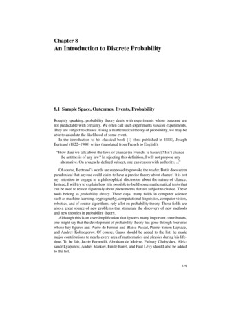
3408 An Introduction to Discrete ProbabilityPr(A B) Pr(A \ B) 1 Pr(B)43 1 .4 3Contrary to the popular belief that Pr(A B) 1/2, it is actually equal to 1/3. Now,consider the question: what is the probability that both are boys given that the firstchild is a boy? The answer to this question is indeed 1/2.The next example is known as the “Monty Hall Problem,” a standard example ofevery introduction to probability theory.Example 8.7. On the television game Let’s Make a Deal, a contestant is presentedwith a choice of three (closed) doors. Behind exactly one door is a terrific prize. Theother doors conceal cheap items. First, the contestant is asked to choose a door. Thenthe host of the show (Monty Hall) shows the contestant one of the worthless prizesbehind one of the other doors. At this point, there are two closed doors, and thecontestant is given the opportunity to switch from his original choice to the otherclosed door. The question is, is it better for the contestant to stick to his originalchoice or to switch doors?We can analyze this problem using conditional probabilities. Without loss of generality, assume that the contestant chooses door 1. If the prize is actually behind door1, then the host will show door 2 or door 3 with equal probability 1/2. However, ifthe prize is behind door 2, then the host will open door 3 with probability 1, and ifthe prize is behind door 3, then the host will open door 2 with probability 1. WritePi for “the prize is behind door i,” with i 1, 2, 3, and D j for “the host opens doorD j, ” for j 2, 3. Here it is not necessary to consider the choice D1 since a sensiblehost will never open door 1. We can represent the sequences of choices occurring inthe game by a tree known as probability tree or tree of possibilities, shown in Figure8.3.Every leaf corresponds to a path associated with an outcome, so the sample spaceisW {P1; D2, P1; D3, P2; D3, P3; D2}.The probability of an outcome is obtained by multiplying the probabilities along thecorresponding path, so we havePr(P1; D2) 16Pr(P1; D3) 16Pr(P2; D3) 131Pr(P3; D2) .3Suppose that the host reveals door 2. What should the contestant do?The events of interest are:1. The prize is behind door 1; that is, A {P1; D2, P1; D3}.2. The prize is behind door 3; that is, B {P3; D2}.3. The host reveals door 2; that is, C {P1; D2, P3; D2}.Whether or not the contestant should switch doors depends on the values of theconditional probabilities1. Pr(A C): the prize is behind door 1, given that the host reveals door 2.
8.2 Conditional Probability and Independence3411/2D2Pr(P 1; D2) 1/61/2D3Pr(P 1; D3) 1/6D3Pr(P 2; D3) 1/3D2Pr(P 3; D2) 1/3P11/31/31P21/31P3Fig. 8.3 The tree of possibilities in the Monty Hall problem.2. Pr(B C): the prize is behind door 3, given that the host reveals door 2.We have A \C {P1; D2}, soPr(A \C) 1/6,andPr(C) Pr({P1; D2, P3; D2}) soPr(A C) Pr(A \C) 1 Pr(C)61 1 1 ,6 3 21 1 .2 3We also have B \C {P3; D2}, soPr(B \C) 1/3,andPr(B C) Pr(B \C) 1 Pr(C)31 2 .2 3Since 2/3 1/3, the contestant has a greater chance (twice as big) to win the biggerprize by switching doors. The same probabilities are derived if the host had revealeddoor 3.A careful analysis showed that the contestant has a greater chance (twice as large)of winning big if she/he decides to switch doors. Most people say “on intuition” thatit is preferable to stick to the original choice, because once one door is revealed,the probability that the valuable prize is behind either of two remaining doors is
3428 An Introduction to Discrete Probability1/2. This is incorrect because the door the host opens depends on which door thecontestant orginally chose.Let us conclude by stressing that probability trees (trees of possibilities) are veryuseful in analyzing problems in which sequences of choices involving various probabilities are made.The next proposition shows various useful formulae due to Bayes.Proposition 8.3. (Bayes’ Rules) For any two events A, B with Pr(A) 0 and Pr(B) 0, we have the following formulae:1. (Bayes’ rule of retrodiction)Pr(B A) Pr(A B)Pr(B).Pr(A)2. (Bayes’ rule of exclusive and exhaustive clauses) If we also have Pr(A) 1 andPr(B) 1, thenPr(A) Pr(A B)Pr(B) Pr(A B)Pr(B).More generally, if B1 , . . . , Bn form a partition of W with Pr(Bi ) 0 (n2), thennPr(A) Â Pr(A Bi )Pr(Bi ).i 13. (Bayes’ sequential formula) For any sequence of events A1 , . . . , An , we have!!Prn\Aii 1 Pr(A1 )Pr(A2 A1 )Pr(A3 A1 \ A2 ) · · · Pr An n\1Ai .i 14. (Bayes’ law)Pr(B A) Pr(A B)Pr(B).Pr(A B)Pr(B) Pr(A B)Pr(B)Proof. By definition of a conditional probability we havePr(A B)Pr(B) Pr(A \ B) Pr(B \ A) Pr(B A)Pr(A),which shows the first formula. For the second formula, observe that we have thedisjoint unionA (A \ B) [ (A \ B),soPr(A) Pr(A \ B) [ Pr(A \ B) Pr(A B)Pr(B) [ Pr(A B)Pr(B).
8.2 Conditional Probability and Independence343We leave the more general rule as an exercise, and the third rule follows by unfoldingdefinitions. The fourth rule is obtained by combining (1) and (2). tuBayes’ rule of retrodiction is at the heart of the so-called Bayesian framework. Inthis framework, one thinks of B as an event describing some state (such as havinga certain disease) and of A an an event describing some measurement or test (suchas having high blood pressure). One wishes to infer the a posteriori probabilityPr(B A) of the state B given the test A, in terms of the prior probability Pr(B) andthe likelihood function Pr(A B). The likelihood function Pr(A B) is a measure ofthe likelihood of the test A given that we know the state B, and Pr(B) is a measureof our prior knowledge about the state; for example, having a certain disease. Theprobability Pr(A) is usually obtained using Bayes’s second rule because we alsoknow Pr(A B).Example 8.8. Doctors apply a medical test for a certain rare disease that has theproperty that if the patient is affected by the disease, then the test is positive in 99%of the cases. However, it happens in 2% of the cases that a healthy patient testspositive. Statistical data shows that one person out of 1000 has the disease. What isthe probability for a patient with a positive test to be affected by the disease?Let S be the event that the patient has the disease, and and the events thatthe test is positive or negative. We know thatPr(S) 0.001Pr( S) 0.99Pr( S) 0.02,and we have to compute Pr(S ). We use the rulePr(S ) We also haveso we obtainPr( S)Pr(S).Pr( )Pr( ) Pr( S)Pr(S) Pr( S)Pr(S),Pr(S ) 0.99 0.0011 5%.0.99 0.001 0.02 0.999 20Since this probability is small, one is led to question the reliability of the test! Thesolution is to apply a better test, but only to all positive patients. Only a small portionof the population will be given that second test becausePr( ) 0.99 0.001 0.02 0.999 0.003.Redo the calculations with the new data
3448 An Introduction to Discrete ProbabilityPr(S) 0.00001Pr( S) 0.99Pr( S) 0.01.You will find that the probability Pr(S ) is approximately 0.000099, so the chanceof being sick is rather small, and it is more likely that the test was incorrect.Recall that in Definition 8.3, we defined two events as being independent ifPr(A \ B) Pr(A)Pr(B).Asuming that Pr(A) 6 0 and Pr(B) 6 0, we havePr(A \ B) Pr(A B)Pr(B) Pr(B A)Pr(A),so we get the following proposition.Proposition 8.4. For any two events A, B such that Pr(A) 6 0 and Pr(B) 6 0, thefollowing statements are equivalent:1. Pr(A \ B) Pr(A)Pr(B); that is, A and B are independent.2. Pr(B A) Pr(B).3. Pr(A B) Pr(A).Remark: For a fixed event B with Pr(B) 0, the function A 7! Pr(A B) satisfiesthe axioms of a probability measure stated in Definition 8.2. This is shown in Ross[11] (Section 3.5), among other references.The examples where we flip a coin n times or roll two dice n times are examplesof indendent repeated trials. They suggest the following definition.Definition 8.5. Given two discrete probability spaces (W1 , Pr1 ) and (W2 , Pr2 ), wedefine their product space as the probability space (W1 W2 , Pr), where Pr is givenbyPr(w1 , w2 ) Pr1 (w1 )Pr2 (W2 ), w1 2 W1 , w2 2 W2 .There is an obvious generalization for n discrete probability spaces. In particular, forany discrete probability space (W , Pr) and any integer n 1, we define the productspace (W n , Pr), withPr(w1 , . . . , wn ) Pr(w1 ) · · · Pr(wn ),wi 2 W , i 1, . . . , n.The fact that the probability measure on the product space is defined as a product of the probability measures of its components captures the independence of thetrials.Remark: The product of two probability spaces (W1 , F1 , Pr1 ) and (W2 , F2 , Pr2 )can also be defined, but F1 F2 is not a s -algebra in general, so some seriouswork needs to be done.
8.3 Random Variables and their Distributions345Next, we define what is perhaps the most important concept in probability: thatof a random variable.8.3 Random Variables and their DistributionsIn many situations, given some probability space (W , Pr), we are more interestedin the behavior of functions X : W ! R defined on the sample space W than in theprobability space itself. Such functions are traditionally called random variables, asomewhat unfortunate terminology since these are functions. Now, given any realnumber a, the inverse image of aX1(a) {w 2 W X(w) a},is a subset of W , thus an event, so we may consider the probability Pr(Xdenoted (somewhat improperly) by1 (a)),Pr(X a).This function of a is of great interest, and in many cases it is the function that wewish to study. Let us give a few examples.Example 8.9. Consider the sample space of 5 coin flips, with the uniform probabilitymeasure (every outcome has the same probability 1/32). Then the number of timesX(w) that H appears in the sequence w is a random variable. We determine that13210Pr(X 3) 32Pr(X 0) 5325Pr(X 4) 32Pr(X 1) 10321Pr(X 5) .32Pr(X 2) The function defined Y such that Y (w) 1 iff H appears in w, and Y (w) 0otherwise, is a random variable. We have13231Pr(Y 1) .32Pr(Y 0) Example 8.10. Let W D D be the sample space of dice rolls, with the uniformprobability measure Pr (every outcome has the same probability 1/36). The sumS(w) of the numbers on the two dice is a random variable. For example,S(2, 5) 7.The value of S is any integer between 2 and 12, and if we compute Pr(S s) fors 2, . . . , 12, we find the following table.
3468 An Introduction to Discrete Probabilitys2 3 4 5 6 7 8 9 10 11 121 2 3 4 5 6 5 4 3 2 1Pr(S s) 3636 36 36 36 36 36 36 36 36 36Here is a “real” example from computer science.Example 8.11. Our goal is to sort of a sequence S (x1 , . . . , xn ) of n distinct realnumbers in increasing order. We use a recursive method known as quicksort whichproceeds as follows:1. If S has one or zero elements return S.2. Pick some element x xi in S called the pivot.3. Reorder S in such a way that for every number x j 6 x in S, if x j x, then x j ismoved to a list S1 , else if x j x then x j is moved to a list S2 .4. Apply this algorithm recursively to the list of elements in S1 and to the list ofelements in S2 .5. Return the sorted list S1 , x, S2 .Let us run the algorithm on the input listS (1, 5, 9, 2, 3, 8, 7, 14, 12, 10).We can represent the choice of pivots and the steps of the algorithm by an orderedbinary tree as shown in Figure 8.4. Except for the root node, every node corresponds(1, 5, 9, 2, 3, 8, 7, 14, 12, 10)1/10(1, 2)3(5, 9, 8, 7, 14, 12, 10)1/2()11/7(2)(5, 7)81/41/2(5)7(9, 14, 12, 10)()(9) 10 (14, 12)1/2() 12 (14)Fig. 8.4 A tree representation of a run of quicksort.to the choice of a pivot, say x. The list S1 is shown as a label on the left of node x,
8.3 Random Variables and their Distributions347and the list S2 is shown as a label on the right of node x. A leaf node is a node suchthat S1 1 and S2 1. If S1 2, then x has a left child, and if S2 2, then xhas a right child. Let us call such a tree a computation tree. Observe that except forminor cosmetic differences, it is a binary search tree. The
An Introduction to Discrete Probability 8.1 Sample Space, Outcomes, Events, Probability Roughly speaking, probability theory deals with experiments whose outcome are not predictable with certainty. We often call such experiments random experiments. They are subject to chance. Using a mathematical theory of probability, we may be