Transcription
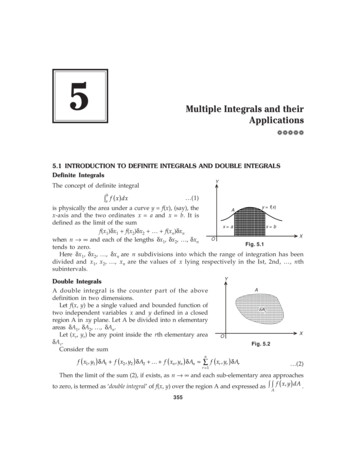
5Multiple Integrals and theirApplicationsaaaaa5.1 INTRODUCTION TO DEFINITE INTEGRALS AND DOUBLE INTEGRALSDefinite IntegralsYThe concept of definite integral a f ( x ) dxb (1)y f( x)is physically the area under a curve y f(x), (say), theAx-axis and the two ordinates x a and x b. It isdefined as the limit of the sumx ax bf(x1)δx1 f(x2)δx2 f(xn)δxnXOwhen n and each of the lengths δx1, δx2, , δxnFig. 5.1tends to zero.Here δx1, δx2, , δxn are n subdivisions into which the range of integration has beendivided and x1, x2, , xn are the values of x lying respectively in the Ist, 2nd, , nthsubintervals.Double IntegralsA double integral is the counter part of the abovedefinition in two dimensions.Let f(x, y) be a single valued and bounded function oftwo independent variables x and y defined in a closedregion A in xy plane. Let A be divided into n elementaryareas δA1, δA2, , δAn.Let (xr, yr) be any point inside the rth elementary areaδA r.Consider the sumYAδA rXOFig. 5.2f ( x1 , y1 ) δ A1 f ( x2 , y2 ) δ A2 f ( xn , yn ) δ An f ( xr , yr ) δ Arn (2)r 1Then the limit of the sum (2), if exists, as n and each sub-elementary area approachesto zero, is termed as ‘double integral’ of f(x, y) over the region A and expressed as f ( x, y ) dA .A355
356Engineering Mathematics through ApplicationsThusLt f ( x, y ) dA n Aδ Ar 0n f ( xr , yr ) δAr (3)r 1Observations: Double integrals are of limited use if they are evaluated as the limit of the sum. However, theyare very useful for physical problems when they are evaluated by treating as successive single integrals.Further just as the definite integral (1) can be interpreted as an area, similarly the double integrals (3) can beinterpreted as a volume (see Figs. 5.1 and 5.2).5.2 EVALUATION OF DOUBLE INTEGRALEvaluation of double integral f ( x, y ) dx dyRy-axisis discussed under following three possible cases:Case I: When the region R is bounded by two continuouscurves y ψ (x) and y φ (x) and the two lines (ordinates)x a and x b.In such a case, integration is first performed withrespect to y keeping x as a constant and then theresulting integral is integrated within the limits x aand x b.Mathematically expressed as:x b(y Ψ (x )y φ( x ) f ( x, y ) dx dy Rx aRy a x θ(y)RAx aOy φ(x)BPx bx axisFig. 5.3)Case 2: When the region R is bounded by two continuouscurves x φ (y) and x Ψ (y) and the two lines (abscissa)y a and y b.In such a case, integration is first performed withrespect to x. keeping y as a constant and then theresulting integral is integrated between the two limitsy a and y b.Mathematically expressed as: f ( x, y ) dx dy y Ψ(x)Df ( x , y ) dy dxGeometrically the process is shown in Fig. 5.3,where integration is carried out from inner rectangle(i.e., along the one edge of the ‘vertical strip PQ’ fromP to Q) to the outer rectangle.y b x Ψ( y)QC f ( x , y ) dx dy Geometrically the process is shown in Fig. 5.4,where integration is carried out from inner rectangle(i.e., along the one edge of the horizontal strip PQfrom P to Q) to the outer rectangle.Case 3: When both pairs of limits are constants, the regionof integration is the rectangle ABCD (say).y axisx Ψ (y)x φ( y )y bBDPQRy aACOx axisFig. 5.4y-axisy aQDRy bOCSAPx aFig. 5.5Bx bx-axis
Multiple Integrals and their Applications357In this case, it is immaterial whether f(x, y) is integrated first with respect to x or y, theresult is unaltered in both the cases (Fig. 5.5).Observations: While calculating double integral, in either case, we proceed outwards from the innermostintegration and this concept can be generalized to repeated integrals with three or more variable also.Example 1: Evaluate1 x 21 00(1dydx1 x2 y2)[Madras 2000; Rajasthan 2005].Solution: Clearly, here y f(x) varies from 0 to 1 x2and finally x (as an independent variable) goes between 0to 1.I 1 1 x21 1 x200 0 y 1 tan 1 0 aa 0 πlog (1 2 )411 x201 x2C(1, 1. 414)(2, 0)O(0, 0)(10) (1. 732, 0)dxFig. 5.62 1 1 x tan 1 0 dx tan2 1 x 1BA(0, 1) 1dy dx , a2 (1 x2)2 a y 1(0, 2)(1. 732, 2) 1dy dx22(1 x ) y 20D (2, 2. 36){}1 π 0 dx π log x 1 x2 1 0 4 1 x2 410Example 2: Evaluate e2x 3y dxdy over the triangle bounded by the lines x 0, y 0 andx y 1.Solution: Here the region of integration is the triangle OABO as the line x y 1 intersectsthe axes at points (1, 0) and (0, 1). Thus, precisely the region R (say) can be expressed as:0 x 1, 0 y 1 – x (Fig 5.7). 2x 3yI edxdyBR1 1 x e2 x 3 y dy dx 0 01 x1 e2 x 3 y dx 00 31Y(0, 1)Qx 1x 0(1, 0)O(0, 0)Py 0AFig. 5.7X
358Engineering Mathematics through Applications (e1 e2x ) dx 13 1 e3 x e2 x 3 12 0 1 2 e2 3 1 e e 3 22 112 2e3 3e2 1 (2e 1)( e 1) . 663 x01Example 3: Evaluate the integral xy ( x y )dxdy over the area between the curves y x2Rand y x.Solution: We have y x2 and y x which impliesx2 – x 0 i.e. either x 0 or x 1Further, if x 0 then y 0; if x 1 then y 1. Means thetwo curves intersect at points (0, 0), (1, 1). The region R of integration is doted and can beexpressed as: 0 x 1, x2 y x. 0 1 xy ( x y ) dxdy R xx2Yy x2Q xy ( x y ) dy dx PO (0, 0)xy3 2 y2 xx dx0 23 x2 y xA(1, 1)X1 Fig. 5.81 x4 x4 x6 x7 dx 0 23 23 6 x10 54 1 6 1 7 x x dx23 11 113 5 x5 1 x7 1 x8 6 5 2 7 3 8 0 6 14 24 56x2 y22Example 4: Evaluate ( x y ) dxdy over the area bounded by the ellipse 2 2 1.ab[UP Tech. 2004, 05; KUK, 2009]Solution: For the given ellipsex2 y2 1 , the region of integration can be considered asa2 b2
Multiple Integrals and their Applicationsbounded by the curves y b 1 x2x2,yb1 and finally x goes from – a to aa2a2I ( x y ) dxdy 2 I [Here a ab 1 x2 / a2 b3591 x2 / a2 –a ab 1 x 2 / a2–b 1 x2 / a2 ( x2 y2 2xy) dy dx ( x2 y2 ) dy dx 2xy dy 0 as it has the same integral value for both limits i.e., the term xy, which isan odd function of y, on integration gives a zero value.]a I 4 0 b 1 x2 / a2Y ( x2 y2 ) dy dxQ 0 y I 4 x2 y 3 0 0 XO223 b 1 x / aadxx –aPx aFig. 5.91322 2 b3 2 xx2I 4 x b 1 2 1 2 dx 3 a a 0 a On putting x a sinθ, dx a cosθ dθ; we get I 4bπ /20 4abb3 223 ( a sin θ cos θ) cos θ a cos θdθ3π /20 2b3224 a sin θ cos θ cos θ dθ3 1 p 1 q 1 π /222 2 sinp x cosq x dx Now using formula 0 p q 2 2 and π /20cosn x dx n 1 2 π,2 n 2 2 3 3 5 1 2( x y )2 dxdy 4ab a2 2 2 b3 2 22323 (in particular when p 0 , q n)
360Engineering Mathematics through Applications 3 ππ ππ 2 2 2b2 2 2 4ab a 2.2.13 2.2.1 1Q π 2 22 πa2 πb2 πab ( a b ) 4ab 16 4 16ASSIGNMENT 1 dx dy1 11. Evaluate(1 x2 )(1 y2 )0 02. Evaluate xy dx dy, where A is the domain bounded by the x-axis, ordinate x 2a andRthe curve x2 4ay.[M.D.U., 2000]3. Evaluate eax by dy dx , where R is the area of the triangle x 0, y 0, ax by 1 (a 0,b 0). [Hint: See example 2]21121331yy4. Prove that ( xy e ) dy dx ( xy e ) dx dy .15. Show that1x y ( x y)dx0 6. Evaluate e310 x2 (1 y2 )1x dx dy00x y ( x y)dy dy03dx .0[Hint: Put x2(1 y2) t, taking y as const.]5.3 CHANGE OF ORDER OF INTEGRATION IN DOUBLE INTEGRALSThe concept of change of order of integration evolved to help in handling typical integralsoccurring in evaluation of double integrals.When the limits of given integral a y φ(x) f ( x, y ) dy dx are clearly drawn and the regionby Ψ( x )of integration is demarcated, then we can well change the order of integration be performingintegration first with respect to x as a function of y (along the horizontal strip PQ from P toQ) and then with respect to y from c to d.Mathematically expressed as:I d cx Ψ ( y)x φ( y )f ( x, y ) dx dy.Sometimes the demarcated region may have to be split into two-to-three parts (as the casemay be) for defining new limits for each region in the changed order.
Multiple Integrals and their Applications3611 x21Example 5: Evaluate the integral y2 dydx by changing the order of integration.00[KUK, 2000; NIT Kurukshetra, 2010]Solution: In the above integral, y on vertical strip (say PQ) varies as a function of x and thenthe strip slides between x 0 to x 1.Here y 0 is the x-axis and y 1 x 2 i.e., x2 y2 1 is the circle.In the changed order, the strip becomes P’Q’, P’ resting on the curve x 0, Q’ on the circlex 1 y 2 and finally the strip P’Q’ sliding between y 0 to y 1.Y 1 y2 2 I y dx dy0 0 1 1I y [ x ]02011 y2QQ P dyy 0XPI y2 (1 1y2 20)dxx 1πSubstitute y sin θ, so that dy cos θ d θ and θ varies from 0 to 2 .x 0Fig. 5.10π2I sin2 θ cos2 θ dθ0I ( 2 1) ( 2 1) π 4 22π16 π Q 2 sinp θ cos θ dθ (p 1)(p 3) (q 1)(q 3) π , only if both p and q are ve even integers] 0(p q)(p q 2) 2 4a2 axdydxby changing the order of integration.Example 6: Evaluate 0 x 24aY[M.D.U. 2000; PTU, 2009]Solution: In the given integral, over the verticalstrip PQ (say), if y changes as a function of x suchx2and Q lies on thethat P lies on the curve y 4acurve y 2 ax and finally the strip slides betweenx 0 to x 4a.x2i.e. x2 4ay is a parabolaHere the curve y 4awith y 0implying x 0 y 4aimplying x 4a (4a, 4a)y2 4axQP AQ x2 4ayPXOx 4aFig. 5.11
362Engineering Mathematics through Applicationsi.e., it passes through (0, 0) (4a, 4a), (– 4a, 4a).Likewise, the curve y 2 ax or y2 4ax is also a parabola withx 0 y 0 and x 4a y 4ai.e., it passes through (0, 0), (4a, 4a), (4a, – 4a).Clearly the two curves are bounded at (0, 0) and (4a, 4a). On changing the order of integration over the strip P’Q’, x changes as a function of ysuch that P’ lies on the curve y2 4ax and Q’ lies on the curve x2 4ay and finally P’Q’ slidesbetween y 0 to y 4a.I whence 4a y2x 4a0 x 2 ay4a[x] y2 ay20 dx dy dy4a4a y2 2 ay 4a dy 04a3 3y2y3 4 a1 2 a 4 a) 2 (( 4a)3 3 12a312a 2 0 32a2 16a2 16a2 .333axa22Example 7: Evaluate x ( x y ) dxdy by changing the order of integration.0aSolution: In the given integral 0 x / a ( x2 a2 ) dx dy , y varies along vertical strip PQ as afunction of x and finally x as an independent variable varies from x 0 to x a.ax /aHere y x/a i.e. x ay is a straight line and y x / a , i.e.x ay2 is a parabola.For x ay; x 0 y 0 and x a y 1.Means the straight line passes through (0, 0), (a, 1).For x ay2; x 0 y 0 and x a y 1.Means the parabola passes through (0, 0), (a, 1), (a, – 1),.Further, the two curves x ay and x ay2 intersect at commonpoints (0, 0) and (a, 1).On changing the order of integration,a 0x/ ax/ aYy x /ay 1QOP Q Px ay2(at P’)Xx a(x2 y2 ) dxdy y 0 x ay (x2 y2 ) dxdy y 1y 0(0, 0)Fig. 5.12
Multiple Integrals and their ApplicationsI 363ay x3 xy2 dy 0 3 ay2 13 ay )3(1 ay.y2 ( ay2 ) ay2 y2 dy 30 3 1 a3 3 a3 64 a y y ay dy 0 33 1 1 a3 y4 a3 y7 ay5 a 43 75 0 3 a3a3 a a 3 4 3 7 4 5 a3aa (5a2 7 ) .28 20 140 aExample 8: Evaluate0y2dy dx.y 4 – a2 x 2aax[SVTU, 2006]Solution: In the above integral, y on the vertical strip (say PQ) varies as a function of x andthen the strip slides between x 0 to x a.Here the curve y ax i.e., y2 ax is the parabola and the curve y a is the straight line.On the parabola, x 0 y 0; x a y a i.e., the parabola passes through points(0, 0), (a, a) and (a, – a).On changing the order of integration, 0a 0 0y2ax 0( at P ) y2a0 ax y2a y2dx dyy4 a2 x2 dx dy2 y2 2 a x 1y2y2 1 x asindy y2 a a 0y-axis(a, a)QP y aQ Py 0O(0, 0)x a x 0I a(a, –a)Fig. 5.13x-axis
364Engineering Mathematics through Applications a a00y2 sin 1 1 sin 1 0 dya y2 ππ y3dy 2a 3a 2a 0πa2.61 2-xExample 9: Change the order of integration of xy dy dx and hence evaluate the same.0 x2[KUK, 2002; Cochin, 2005; PTU, 2005; UP Tech, 2005; SVTU, 2007]1 2 x Solution: In the given integral xydy dx, on the vertical strip PQ(say), y varies as a2 0 xYfunction of x and finally x as an independent variable,varies from 0 to 1.y 2B(0, 2)Here the curve y x2 is a parabola withy 0implying x 0 Q y 1 implying x 1 i.e., it passes through (0, 0), (1, 1), (– 1, 1).Likewise, the curve y 2 – x is straight linewithy 0 x 2 y 1 x 1 y 2 x 0 Q P y x2ACP Q y 1y 2–xy 0POx 0(1, 1)(2, 0)Xx 1Fig. 5.14i.e. it passes though (1, 1), (2, 0) and (0, 2)On changing the order integration, the area OABO is divided into two parts OACO andABCA. In the area OACO, on the strip P’Q’, x changes as a function of y from x 0 to x y .Finally y goes from y 0 to y 1.Likewise in the area ABCA, over the strip p”Q”, x changes as a function of y from x 0 tox 2 – y and finally the strip P”Q” slides between y 1 to y 2. 1 y 2 2 y 0 0 1 0 xy dx dy xy dx dy x2 y20 1 2 x2 dy y 2 1y 0y2dy 2y (2 y)dy22 1 1 2 4y3 y4 2y 6 2 34 10 0 1212I 1 53 .6 24 8 dy 2 y
Multiple Integrals and their Applications2– x2 1Example 10: Evaluate0xxdydx by changing order of integration.x y2[KUK, 2000; MDU, 2003; JNTU, 2005; NIT Kurukshetra, 2008]2YSoluton: Clearly over the strip PQ, y varies as afunction of x such that P lies on the curve y x and Qlies on the curve y 2 x 2 and PQ slides betweenordinates x 0 and x 1.y xMbetween y 0 to y 1 and y 1 to y vely.whenceNow the exp. 1y0 0O 212 y20Q y N (1, 1)2y 1Q Py 0Xx2 y2 2x 1x 02 respecti-xdx dy x2 y2QP LP The curves are y x, a straight line and y 2 x2 ,i.e. x2 y2 2, a circle.The common points of intersection of the two are(0, 0) and (1, 1).On changing the order of integration, the sameregion ONMO is divided into two parts ONLO andLNML with horizontal strips P’Q’ and P”Q” slidingI 365Fig. 5.15xdx dyx2 y21xd 22 2xy ()x2 y2 dxI I 1 ( x201 ( x20)1ay a 1 y y2 2 0)dy 2dy 2111 2( x y2 )2 02 y21 2( x y2 )2 02 y2dydy2y2y2 12 1) 2 y ( 2 1)2 0 2 02(Example 11: Evaluate 1 y y2 2 0 0a a2 – y2a a2 – y2dy dx by changing the order of integration. dx dyy ox a Clearly in the region under consideration, strip PQ is horizontal with point P lying on theSolution: Given x a a 2 y 2a 2 y2curve x a a2 y 2 and point Q lying on the curve x a a2 y2 and finally this stripslides between two abscissa y 0 and y a as shown in Fig 5.16.
366Engineering Mathematics through ApplicationsYx 0Now, for changing the order of integration, theregion of integration under consideration is same butthis time the strip is P’Q’ (vertical) which is a functionof x with extremities P’ and Q’ at y 0 andy 2ax x2 respectively and slides between x 0and x 2a.2a 2ax x2I 0 Thus 02ax x2a dxdy dx y 0022a2a00CQ' x 2aQPA(0, 0)O(a, 0) 2ax x2 dx x 2a x dx2a sin θ so that dx 4a sinθ cos θ dθ,πFor x 0, θ 0 and for x 2a, θ 2Also,Xx2 y2 2axx TakeB (2a, 0)P'Fig. 5.16π2I 2a sin θ 2a 2a sin2 θ 4a sin θ cos θ dθTherefore,0π2 8a2 sin 2 θ cos2 θ dθ 8a2 0(2 1)(2 1) π πa24 ( 4 2) 22 using sinp θ cosq θ dθ (p 1)(p 3) (q 1)(q 3) π , (p q)(p q 2) 20 p and q both positive even integers π23 4 yExample 12: Changing the order of integration, evaluate 01( x y ) dx dy.[MDU, 2001; Delhi, 2002; Anna, 2003; VTU, 2005]Solution: Clearly in the given form of integral, xchanges as a function of y (viz. x f(y) and y as anindependent variable changes from 0 to 3.Thus, the two curves are the straight line x 1 andthe parabola, x 4 y and the common area underconsideration is ABQCA.For changing the order of integration, we need toconvert the horizontal strip PQ to a vertical strip P’Q’over which y changes as a function of x and it slides forvalues of x 1 to x 2 as shown in Fig. 5.17. I 2 1( 4 x2 )0 ( x y ) dy dx 2 1C (1, 3)dxy 3Q'QPOAP Fig. 5.174 x2y2 xy 2 0 YB y 0(2, 0)X
Multiple Integrals and their Applications 2 x ( 4 x2 ) 1 367( 4 x2 )2 dx 22 x4 248xx 4x2 dx() 2 12 x4x5 4 3 2x2 8x x410 3 1 2 ( 22 12 ) 6 1 4( 2 14 ) 8 (2 1) 101 ( 25 15 ) 34 (23 13 )41531 28 241. 8 410 360a2Example 13: Evaluate 00a2 y 2()log x 2 y 2 dx dy ( a 0 ) changing the order of integration.[MDU, 2001]Solution: Over the strip PQ (say), x changes as a function of y such that P lies on the curveYx2 y2 a2 x y and Q lies on the curve x a2 y2 anda .the strip PQ slides between y 0 to y 2Here the curves, x y is a straight lineBx 0 y 0 aa x y 22 andxyQ PGHaa,2,2JKy Q Qy 0O(0, 0) aa , i.e. it passes through (0, 0) and 22 P P Aa2Xx aAlso x a2 y2 , i.e. x2 y2 a2 is a circlewith centre (0, 0) and radius a.x 0 aa ,Thus, the two curves intersect at .22 x a2Fig. 5.18On changing the order of integration, the same region OABO is divided into two partswith vertical strips P’Q’ and P”Q” sliding between x 0 to x aaand x to x a22respectively.Whence,I a/ 20 x0log ( x2 y2 ) dy dx aa/ 2 0a2 x2 log ( x2 y2 ) 1 dy dx (1)
368Engineering Mathematics through ApplicationsNow, log ( x2IstFunction y2 ) 1 dy log ( x2 y2 ) y x2 12y y dy 2 y IIndFunction y2 x2 x2 dy y log ( x2 y2 ) 2x2 y2 y log ( x2 y2 ) 2 y 2x2 1dy ( x2 y2 ) y 1 y log ( x2 y2 ) 2y 2x2 tan 1 xx (2)On using (2),I1 a/ 2 a/ 2 a/ 2 a/ 20000x 22 1 y y log ( x y ) 2y 2x tan x dx 0 x log 2x2 2x 2x tan 1 1 dx x log 2x2 2x 2x π dx 4 πx log 2x2 dx 2 1 4 a/ 20x dxFor first part, let 2x2 t so that 4x dx dt and limits are t 0 and t a2. I1 a20a/ 20a21 π 1 a2t ( log t 1) 0 4 2 , (By parts with logt logt · 1)4 2πlog t dt 2 1 x 4 24a2π a2 a2log a2 1) (482 (3)Agian, using (2),I2 aa/ 2 aa/ 2 22 1 y y log ( x y ) 2y 2x tan x 0a2 x2dx22 2 1 a x2222 a x log a 2 a x 2x tanx (4) dx
Multiple Integrals and their Applicationsππto42Let x a sinθ so that dx a cos θ dθ and limits, I2 π/ 2π/ 4 π /2π/4222 2222 1 a a sin θ (log a 2) a a sin θ 2a sin θ tan a cos θ dθa sin θ a2 (log a2 2) cos2 θ dθ a2 a2 ( log a2 2 ) 369 π /2π /4 π /2π/42 sin θ cos θ tan 1 (cot θ) dθ(1 cos 2θ) dθ a22π /2sin 2θ a2log a2 2 ) θ a2(24 π/4 π /2π /4π /2π /4 π sin 2θ tan 1 tan θ dθ 2 π θ sin 2θ dθ 2 IstFun.IIndFun.π /2 π π 1 a2 cos 2θ 22 πaalog2 ( ) θ 22 π/4 2 4 2 2a2a2π 1log a2 2) ( 4 2 22I2 π /2π /4 π /2π /4 ( 1) cos 2θ dθ 2 π cos 2θ cos 2θ dθ , θ is zero for both 2 2 the limits)π π a2π a2 a2 a2 a2log a2 log a2 (sin 2θ)π 2 8 44424 π a2π a2 a2 a2 a2log a2 log a2 8 4424 (5)On using results (3) and (5), we getI I1 I2 a2a2 πa2 a2 πa2πa2 a2 a2a2 log a2 log a2 log a2 4482 84244 πa2πa2 πa2log a2 (log a2 1)888 1πa2πa2 2 log a 1) log a .(84 2 xExample 14: Evaluate by changing the order of integration. xe– x 2 /ydx dy00[VTU, 2004; UP Tech., 2005; SVTU, 2006; KUK, 2007; NIT Kurukshetra, 2007]
370Engineering Mathematics through Applications Solution: We write0x0xe x2 /ydxdy x ( b )y f2 ( x ) xx 0( ay f1 (x ) 0 ) xe x2/ydxdyHere first integration is performed along the vertical strip with y as a function of x andthen x is bounded between x 0 to x .We need to change, x as a function of y and finally the limits of y. Thus the desiredgeometry is as follows:In this case, the strip PQ changes to P’Q’ with x as function of y, x1 y and x2 andfinally y varies from 0 to .Therefore Integtral I xe x2/ydxdy0 yPut x2 t so that 2x dx dt Further, forI 0y 1 2 x y , t y2 , x , t Qdtdy,2 e t / y dy 1/ y y2 e t/ y2 O1 e y y 2 1 0 1 ye y e y 02 11 (0) (0 1) .2 21 e y dy 1 0 e –ydy dx.x –y0[NIT Jalandhar, 2004, 2005; VTU, 2007]Example 15: Evaluate the integral Soluton: In the given integral, integration is performed firstwith respect to y (as a function of x along the vertical strip sayPQ, from P to Q) and then with respect to x from 0 to .On changing the order, of integration integration isperformed first along the horizontal strip P'Q' (x as a functionof y) from P' to Q' and finally this strip P'Q' slides betweenthe limits y 0 to y .YQy xx Q P x 0 0Fig. 5.19 XP Q'P' y 0 e y dy02 ye y dy (By parts)020YPy 0O (0, 0)Fig. 5.20X
Multiple Integrals and their ApplicationsI ye y 0 e y 10 y0 dx dy e y( y ) dy y 0371 0e y dy11 1 0 ee – 1(0 – 1) 1Example 16: Change the order of integration in the double integral 2a0[Rajasthan, 2006; KUK, 2004-05]0x 2 2axf ( x , y) dydx aa a 2 y20y 2 /2 a y 2a 2a0a a2 y2 Part IIf ( x, y) dydx Q x 0P ΙΙΙΙP PP Q ΙΙy aQ (a , 0)y 0O(0, 0)Xf ( x, y) dydx( x – a) 2 y2 a22a2aay 2 / 2a Fig. 5.21f ( x, y) dydxYPart IIIExample 17: Find the area bounded by the lines y sin x, y cos x and x 0.QSolution: See Fig 5.22.Clearly the desired area is the doted portionwhere along the strip PQ, P lies on the curvey sin x and Q lies on the curve y cos x and finallythe strip slides between the ordinates x 0 andP π 1 , 4 2 y sinxOx 0πx .4Qy2 2 axPart Iaf ( x, y ) dx dy.x 2a 2ax2ax - x2YSolution: Clearly from the expressions given above,the region of integration is described by a line whichstarts from x 0 and moving parallel to itself goesover to x 2a, and the extremities of the moving linelie on the parts of the circle x2 y2 – 2ax 0 the parabolay2 2ax in the first quadrant.For change and of order of integration, we need toconsider the same region as describe by a line movingparallel to x-axis instead of Y-axis.In this way, the domain of integration is dividedinto three sub-regions I, II, III to each of whichcorresponds a double integral.Thus, we get2a2axπ2πy cosxFig. 5.223π22πX
372Engineering Mathematics through Applicationsπ4 cos x dx dy dy dx R0sin xπ4 (cos x sin x) dx0 (sin x cos x )0π /4 1 1 0 1 . 2 2 ()2 1ASSIGNMENT 2 a1. Change the order of integration0ayxdxdyx y22aa2 y22. Change the order integration in the integral a 0a cos α3. Change the order of integration in 4. Change the order of integration in a2 x 2x tan α0alx0mxf ( x, y ) dx dyf ( x , y ) dy dxf (x, y)dxdy[PTU, 2008]5.4 EVALUATION OF DOUBLE INTEGRAL IN POLAR COORDINATESθ β r Ψ(θ)To evaluate θ α r φ(θ )f ( r, θ) dr dθ, we first integrate with respect to r between the limitsr φ(θ) to r ψ(θ) keeping θ as a constant and then theresulting expression is integrated with respect to θ from θ α to θ β.θ r Ψ(θ)r Ψ(θ)Dr φ(θ)Geometrical Illustration: Let AB and CD be the twocontinuous curves r φ(θ) and r Ψ(θ) bounded betweenthe lines θ α and θ β so that ABDC is the requiredregion of integration.Let PQ be a radial strip of angular thickness δθ when OPmakes an angle θ with the initial line.Here r φ(θ) f ( r, θ) dr refers to the integration withπ2QCδθPθ βBθθ αθ 0Orespect to r along the radial strip PQ and then integrationwith respect to θ means rotation of this strip PQ from AC to CD.AFig. 5.23
Multiple Integrals and their Applications373θ) above the initial line.Example 18: Evaluate r sinθ dr dθ over the cardiod r a (1 – cosθSolution: The region of integration under consideration is the cardiod r a(1 – cos θ) abovethe initial line.In the cardiodr a(1 – cos θ); forθ 0, r 0, πθ , r a, 2 θ π, r 2a As clear from the geometry along the radial strip OP, r (as a function of θ) varies fromr 0 to r a(1 – cos θ) and then this strip slides from θ 0 to θ π for covering the area abovethe initial line.Henceθ π/2π r a(1 cos θ) I r dr sin θ dθ 0 0A(a , π/2)Pπ 2 a(1 cos θ ) r sin θ dθ0 2 0 θ π CFig. 5.24 f n 1 ( x ) n Q f ( x ) f ( x ) dx n 1 r2sinθ dr dθ R2a3θ above, where R is the semi circle r 2a cosθ3θ π/2Solution: The region R of integration is the semi-circler 2a cos θ above the initial line.For the circler 2a cosθ, θ 0 r 2a r 2a cosθ πθ r 0 2 Otherwise also,θ 04a2a2 a231 cos π ) (1 cos 0) [ 8 0 ] .( 66 3Example 19: Show thatthe initial line.π (1 cos θ)3 ,3 0O(0, 0)(2a, π)a2 π2 (1 cos θ ) sin θ dθ2 0a2 2θBθ 0θ(0, 0)O(a, 0)r 2a cosθ r2 2ar cosθx 2 y2 2ax(x2 – 2ax a2) y2 a2(x – a)2 (y – 0)2 a2Fig. 5.25(2a, 0)
374Engineering Mathematics through Applicationsi.e., it is the circle with centre (a, 0) and radius r aπ2 2 a cos θ2r sin θdr dθHence the desired area 0 0π2 2a cos θ r2 dr sin θdθ 0 0 π /2 r3 3 0π /22 a cos θ0 sin θdθ 13 8a 3 cos 4 θ 3 4 0 , using 2a 3.3Example 20: Evaluate 0(2a)3 cos3 θ sin θ dθπ /2 n 1f (x) f (x) f '(x)dx n 1nr dr dθθ.over one loop of the lemniscate r2 a2 cos2θa2 r 2[KUK, 2000; MDU, 2006]πand maximum value of r is a.4See Fig. 5.26, in one complete loop, r varies from 0 to r a cos 2θ and the radial stripππ.slides between θ to44Hence the desired areaSolution: The lemniscate is bounded for r 0 implying θ π/ 4A π /4 2a cos 2θ0π /4 π/4 ( a2 r2 ) π /4r(a π /4 0 /4 π a cos2θ1 r2 )12dr dθθd ( a2 r2 )12a cos2θ2 dr dθ dθπ /4( ( π /44π/P(r, θ)θ 0Oθ 0) a 2 a 2 cos 2θ 1 2 a d θ π /4 a )2 cos θ 1 dθFig. 5.26–π/4
Multiple Integrals and their Applicationsπ /4 ( 2a)2 cos θ 1 dθ0 2a (3752 sin θ θ)0π/4 1 π π 2a 2 2a 1 . 2 4 4 θ andExample 21: Evaluate r 3 dr dθ , over the area included between the circles r 2a cosθθ (b a).r 2b cosθ[KUK, 2004]Solution: Given r 2a cosθ or r2 2a r cosθx2 y2 2ax(x a)2 (y – 0)2 a2i.e this curve represents the circle with centre (a, 0) and radius a.Likewise, r 2b cosθ represents the circle with centre (b, 0) and radius b.We need to calculate the area bounded between the two circles, where over the radialstrip PQ, r varies from circle r 2b cosθ to r 2a cosθ and finally θ varies from π22 a cos θ3Thus, the given integral r3 dr dθ R r dr dθπ 2b cos θ2θ π214 r 2 b cosθQ4 2a cos θ r dθ π /2 4 2b cos θ π /2ππto .22π /2 ( 2a cos θ)4 ( 2b cos θ)4 dθ π /2 PθO(0, 0)2b2aπ2 4 ( a4 b4 ) cos4 θ dθ π2π2r 2a cos θFig 5. 27 8 ( a4 b4 ) cos4 θ dθ 8 (a b4 40) 43 12 π23π ( a4 b4 ) .2Particular Case: When r 2 cosθ and r 4 cosθ i.e., a 2 and b 1, then3345πunits .I π ( a4 b4 ) π ( 24 14 ) 222
376Engineering Mathematics through ApplicationsASSIGNMENT 31. Evaluate r sin θ dr dθ over the area of the caridod r a(1 cosθ) above the initial line. Hint : I π 0a (1 cos θ )0 r sin θ dr dθ 2. Evaluate r3 dr dθ , over the area included between the circles r 2a cosθ and r 2b cosθ(b a).[Madras, 2006]π 2 r 2b cos θ Hint : I r 3 dr dθ (See Fig. 5.27 with a and b interchanged) π r 2a cos θ 2 3. Find by double integration, the area lying inside the cardiod r a(1 cosθ) and outsidethe parabola r(1 cosθ) a.[NIT Kurukshetra, 2008] Hint : 2 π /2 0 a(1 cos θ)a1 cos θ rdr dθ 5.5 CHANGE OF ORDER OF INTERGRATION IN DOUBLE INTEGRAL IN POLARCOORDINATESθ β r Ψ(θ )In the integral θ α r φ (θ) f ( r, θ) dr dθ , interation is first performed with respect to r along a‘radial strip’ and then this trip slides between two values of θ α to θ β.In the changed order, integration is first performed with respect to θ (as a function of ralong a ‘circular arc’) keeping r constant and then integrate the resulting integral with respectto r between two values r a to r b (say)Mathematically expressed as( )() θ α r φ(θ) f ( r, θ) dr dθ I r a θ f (r) f (r, θ ) dθ drθ β r Ψ θr b θ η rπ /2 2a cosθExample 22: Change the order of integration in the integral 0 0Solution: Here, integration is first performed withrespect to r (as a function of θ) along a radial stripOP (say) from r 0 to r 2a cos θ and finally thisradial strip slides between θ 0 to θ y2a)2y2r 2a cosθ or θ cos 1a2O(0, 0)r2aPR 2ax (x – i.e., it is circle with centre (a, 0) and radius a.On changing the order of integration, we have tofirst integrate with respect to θ (as a function of r) alongx2π2π.2r 2a cosθ r2 2a rcosθCurveθ f ( r , θ ) dr dθθQ (a , 0)(2 a, 0)x 2aFig. 5.28θ 0
Multiple Integrals and their Applications377 1 rthe ‘circular strip’ QR (say) with pt. Q on the curve θ 0 and pt. R on the curve θ cos2aand finally r varies from 0 to 2a.π2I cos 1 2r a f ( r, θ) dr dθ f (r, θ) dθ dr 0 02a cos θ 002aπExample 23: Sketch the region of integrationaeπ / 4 π /22 log ra0π /2a2log of integration.Solution: Double integralae 4raf ( r , θ ) r dr dθ and change the orderr βf ( r, θ) r dr dθ is identical to r αθ f2(r)f (r, θ)rdrdθ, whence θ f1(r)integration is first performed with respect to θ as a function of r i.e., θ f(r) along ther‘circular strip’ PQ (say) with point P on the curve θ 2 log and point Q on the curveaπθ and finally this strip slides between between r a to r aeπ/4. (See Fig. 5.29).2rθrThe curve θ 2 log implies logaa2reθ/2 or r a eθ/2aNo
Multiple Integrals and their Applications 357 In this case, it is immaterial whether f(x, y) is integrated first with respect to x or y, the result is unaltered in both the cases (Fig. 5.5). Observations:While calculating double integral, in either case, we proceed outwards from the innermost integration and this concept can be generalized to repeated integrals with three or more variable also.