Transcription
5Path Integrals in Quantum Mechanics andQuantum Field TheoryIn chapter 4 we discussed the Hilbert space picture of Quantum Mechanicsand Quantum Field Theory for the case of a free relativistic scalar fields.Here we will present the Path Integral picture of Quantum Mechanics andof relativistic scalar field theories.The Path Integral picture is important for two reasons. First, it offersan alternative, complementary, picture of Quantum Mechanics in which therole of the classical limit is apparent. Secondly, it gives a direct route to thestudy regimes where perturbation theory is either inadequate or fails completely. In Quantum mechanics a standard approach to such problems isthe WKB approximation, of Wentzel, Kramers and Brillouin. However, as ithappens, it is extremely difficult (if not impossible) the generalize the WKBapproximation to a Quantum Field Theory. Instead, the non-perturbativetreatment of the Feynman path integral, which in Quantum Mechanics isequivalent to WKB, is generalizable to non-perturbative problems in Quantum Field Theory. In this chapter we will use path integrals only for bosonicsystems, such as scalar fields. In subsequent chapters we will also give afull treatment of the path integral, including its applications to fermionicfields, abelian and non-abelian gauge fields, classical statistical mechanics,and non-relativistic many body systems.There is a huge literature on path integrals, going back to the originalpapers by Dirac (Dirac, 1933), and particularly Feynman’s 1942 PhD Thesis(Feynman, 2005), and his review paper (Feynman, 1948). Popular textbookson path integrals include the classic by Feynman and Hibbs (Feynman andHibbs, 1965), and Schulman’s book (Schulman, 1981), among many others.
5.1 Path Integrals and Quantum Mechanics1155.1 Path Integrals and Quantum MechanicsConsider a simple quantum mechanical system whose dynamics can be described by a generalized coordinate operator q̂. We want to compute theamplitudeF (qf , tf qi , ti ) ⟨qf , tf qi , ti ⟩(5.1)known as the Wightman function. This function represents the amplitudeto find the system at coordinate qf at the final time tf knowing that it wasat coordinate qi at the initial time ti . The amplitude F (qf , tf qi , ti ) is justa matrix element of the evolution operatoriĤ(ti tf )/h̵F (qf , tf qi , ti ) ⟨qf e qi ⟩(5.2)Let us set, for simplicity, qi , ti ⟩ 0, 0⟩ and qf , tf ⟩ q, t⟩. Then, from thedefinition of this matrix element, we find out that it obeyslim F (q, t 0, 0) ⟨q 0⟩ δ(q)t 0(5.3)Furthermore, after some algebra we also find thatih̵ F iĤt/h̵ ih̵ ⟨q, t 0, 0⟩ ih̵ ⟨q e 0⟩ t t t iĤt/h̵ ⟨q Ĥe 0⟩ dq ⟨q Ĥ q ⟩⟨q e′′′ iĤt/h̵ 0⟩(5.4)where we have used that, since { q⟩} is a complete set of states, the identityoperator I has the expansion, called the resolution of the identity,I dq q ⟩⟨q ′′′(5.5)Here we have assumed that the states are orthonormal,⟨q q ⟩ δ(q q )′Hence,ih̵′ ′′′F (q, t 0, 0) dq ⟨q Ĥ q ⟩F (q , t 0, 0) Ĥq F (q, t 0, 0) t(5.6)(5.7)In other words, F (q, t 0, 0) is the solution of the Schrödinger Equation thatsatisfies the initial condition of Eq. (5.3). For this reason, the amplitudeF (q, t 0, 0) is called the Schrödinger Propagator.
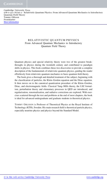
116Path Integrals in Quantum Mechanics and Quantum Field Theory(qf , tf )qfq(q , t )′′qi(qi , ti )tit′′tftFigure 5.1 The amplitude to go from qi , ti ⟩ to qf , tf ⟩ is a sum of products′ ′of amplitudes through the intermediate states q , t ⟩.The superposition principle tells us that the amplitude to find the systemin the final state at the final time is the sum of amplitudes of the formF (qf , tf qi , ti ) dq ⟨qf , tf q , t ⟩⟨q , t qi , ti ⟩′′′′′(5.8)′where the system is in an arbitrary set of states at an intermediate time t .Here we represented this situation by inserting the identity operator I at′the intermediate time t in the form of the resolution of the identity of Eq.(5.8).Let us next define a partition of the time interval [ti , tf ] into N subintervals each of length t,tf ti N t(5.9)ti t0 t1 . . . tN tN 1 tf(5.10)Let {tj }, with j 0, . . . , N 1, denote a set of points in the interval [ti , tf ],such thatClearly, tk t0 k t, for k 1, . . . , N 1. By repeating the procedure usedin Eq.(5.8) of inserting the resolution of the identity at the intermediatetimes {tk }, we findF (qf , tf qi , ti ) dq1 . . . dqN ⟨qf , tf qN , tN ⟩⟨qN , tN qN 1 , tN 1 ⟩ . . . . . . ⟨qj , tj qj 1 , tj 1 ⟩ . . . ⟨q1 , t1 qi , ti ⟩(5.11)
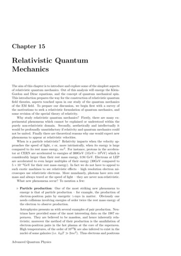
5.1 Path Integrals and Quantum MechanicsEach factor ⟨qj , tj qj 1 , tj 1 ⟩ in Eq.(5.11) has the form iĤ(tj tj 1 )/h̵⟨qj , tj qj 1 , tj 1 ⟩ ⟨qj e qj 1 ⟩ ⟨qj e iĤ t/h̵117 qj 1 ⟩(5.12)In the limit N , with tf ti fixed and finite, the interval t becomesinfinitesimally small and t 0. Hence, as N we can approximatethe expression for ⟨qj , tj qj 1 , tj 1 ⟩ in Eq.(5.12) as follows⟨qj , tj qj 1 , tj 1 ⟩ ⟨qj e qj 1 ⟩ t2 ⟨qj {I i ̵ Ĥ O(( t) )} qj 1 ⟩h t2 δ(qj qj 1 ) i ̵ ⟨qj Ĥ qj 1 ⟩ O(( t) )h iH t/h̵(5.13)which becomes asymptotically exact as N .q(t)qftqititf tFigure 5.2 A history q(t) of the system.We can also introduce at each intermediate time tj a complete set ofmomentum eigenstates { p⟩} using their resolution of the identityI dp p⟩⟨p Recall that the overlap between the states q⟩ and p⟩ is⟨q p⟩ 12π h̵For a typical Hamiltonian of the formipq/h̵e(5.14)(5.15)2Ĥ p̂ V (q̂)2m(5.16)
118Path Integrals in Quantum Mechanics and Quantum Field Theoryits matrix elements are⟨qj Ĥ qj 1⟩ 2pjdpj ipj (qj qj 1 )/h̵e[ V (qj )]̵2m2π h(5.17)Within the same level of approximation we can also writepjdpjqj qj 1[i())](pexp(q q) tH,jj 1j22π h̵h̵(5.18)where we have introduce the “mid-point rule” which amounts to the replacement qj 12 (qj qj 1 ) inside the Hamiltonian H(p, q). Putting everythingtogether we find that the matrix element ⟨qf , tf qi , ti ⟩ becomes⟨qj , tj qj 1 , tj 1 ⟩ ⟨qf , tf qi , ti ⟩ lim dqj NN N 1 j 1dpj2π h̵ N 1 qj qj 1 i )][p(pexp j (qj qj 1 ) t H j , ̵2h j 1 (5.19)j 1Therefore, in the limit N , holding ti tf fixed, the amplitude⟨qf , tf qi , ti ⟩ is given by the (formal) expressioni tf̵ dt [pq̇ H(p, q)]⟨qf , tf qi , ti ⟩ DpDq e h ti(5.20)where we have used the notationNDpDq lim N j 1dpj dqj2π h̵(5.21)which defines the integration measure. The functions, or configurations,(q(t), p(t)) must satisfy the initial and final conditionsq(ti ) qi ,q(tf ) qf(5.22)Thus the matrix element ⟨qf , tf qi , ti ⟩ can be expressed as a sum over histories in phase space. The weight of each history is the exponential factorof Eq. (5.20). Notice that the quantity in brackets it is just the LagrangianL pq̇ H(p, q)(5.23)
5.1 Path Integrals and Quantum Mechanics119Thus the matrix element is just⟨qf , tf q, t⟩ DpDq e h̵iS(q,p)(5.24)where S(q, p) is the action of each history (q(t), p(t)). Also notice thatthe sum (or integral) runs over independent functions q(t) and p(t) whichare not required to satisfy any constraint (apart from the initial and finalconditions) and, in particular they are not the solution of the equationsof motion. Expressions of these type are known as path-integrals. They arealso called functional integrals, since the integration measure is a sum over aspace of functions, instead of a field of numbers as in a conventional integral.Using a Gaussian integral of the form (which involves an analytic continuation)p t t 2i ̵ q̇) ̵dp i(pq̇ m2mhee 2h ̵2π h̵2πih t2 (5.25)we can integrate out explicitly the momenta in the path-integral and find aformula that involves only the histories of the coordinate alone. Notice thatthere are no initial and final conditions on the momenta since the initial andfinal states have well defined positions. The result is⟨qf , tf qi , ti ⟩ Dq ei tf dt L(q, q̇)h̵ ti(5.26)which is known as the Feynman Path Integral (Feynman, 2005, 1948). HereL(q, q̇) is the Lagrangian,1 2L(q, q̇) mq̇ V (q)2(5.27)and the sum over histories q(t) is restricted by the boundary conditionsq(ti ) qi and q(tf ) qf .The Feynman path-integral tells us that in the correspondence limit, h̵ 0, the only history (or possibly histories) that contribute significantly tothe path integral must be those that leave the action S stationary since,otherwise, the contributions of the rapidly oscillating exponential would addup to zero. In other words, in the classical limit there is only one history qc (t)that contributes. For this history, qc (t), the action S is stationary, δS 0,and qc (t) is the solution of the Classical Equation of Motion Ld L 0 qdt q̇(5.28)
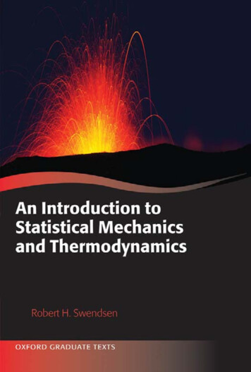
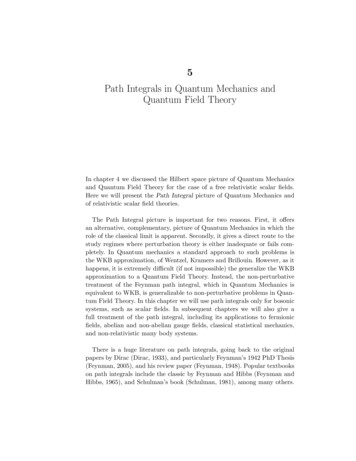
120Path Integrals in Quantum Mechanics and Quantum Field Theoryq(tf )qtiq(ti )tftFigure 5.3 Two histories with the same initial and final states.In other terms, in the correspondence limit h̵ 0, the evaluation of theFeynman path integral reduces to the requirement that the Least ActionPrinciple should hold. This is the classical limit.5.2 Evaluating path integrals in Quantum MechanicsLet us first discuss the following problem. We wish to know how to computethe amplitude ⟨qf , tf qi , ti ⟩ for a dynamical system whose Lagrangian hasthe standard form of Eq. (5.27). For simplicity we will begin with a linearharmonic oscillator.The Hamiltonian for a linear harmonic oscillator is22pmω 2H q2m2and the associated Lagrangian is(5.29)2L m 2 mω 2q̇ q22(5.30)Let qc (t) be the classical trajectory. It is the solution of the classical equations of motion2d qc2 ω qc 0(5.31)2dtLet us denote by q(t) an arbitrary history of the system and by ξ(t) itsdeviation from the classical solution qc (t). Since all the histories, includingthe classical trajectory qc (t), obey the same initial and final conditionsq(ti ) qiq(tf ) qf(5.32)
5.2 Evaluating path integrals in Quantum Mechanics121it follows that ξ(t) obeys instead vanishing initial and final conditions:ξ(ti ) ξ(tf ) 0(5.33)After some trivial algebra it is easy to show that the action S for an arbitraryhistory q(t) becomestfddqcd qc2[mξ] dt mξ ( 2 ω qc )dtdtdttiti(5.34)The third term vanishes due to the boundary conditions obeyed by thefluctuations ξ(t), Eq. (5.33). The last term also vanishes since qc is a solutionof the classical equation of motion Eq. (5.31). These two features hold forall systems, even if they are not harmonic. However, the Lagrangian (andhence the action) for ξ, the second term in Eq. (5.34), in general is not thesame as the action for the classical trajectory (the first term). Only for the has the same form as S(qc , q̇c ).harmonic oscillator S(ξ, ξ)Hence, for a harmonic oscillator, we get the path integral S(q, q̇) S(qc , q̇c ) S(ξ, ξ)⟨qf , tf qi , ti ⟩ e h̵i2tfS(qc ,q̇c )dt ξ(ti ) ξ(tf ) 0iDξ e h̵ ti dtL(ξ,ξ̇)tf(5.35)Notice that the information on the initial and final states enters only throughthe factor associated with the classical trajectory. For the linear harmonicoscillator, the quantum mechanical contribution is independent of the initialand final states. Thus, we need to do two things: 1) we need an explicit solution qc (t) of the equation of motion, for which we will compute S(qc , q̇c ), and2) we need to compute the quantum mechanical correction, the last factorin Eq. (5.35), which measures the strength of the quantum fluctuations.For a general dynamical system, whose Lagrangian has the form of Eq.(5.27), the action of Eq. (5.34) takes the form qc )S(q, q̇) S(qc , q̇c ) Seff (ξ, ξ; tfdtti2tfd V 999dqd q[mξ c ] dt (m 2c 9 ) ξ(t)dtdt q 999qcdtti(5.36)where the Seff is the effective action for the fluctuations ξ(t) which has theformSeff (ξ, ξ̇) tftitf99 V1 2 1 tf′99 ξ(t)ξ(t′ ) O(ξ 3 )dt mξ̇ dt dt′22 ti q(t) q(t ) 99qcti(5.37)2
122Path Integrals in Quantum Mechanics and Quantum Field TheoryOnce again, the boundary conditions ξ(ti ) ξ(tf ) 0 and the fact theqc (t) is a solution of the equation of motion together imply that the last twoterms of Eq. (5.36) vanish identically.3Thus, to the extent that we are allowed to neglect the O(ξ ) corrections(and higher), the effective action Seff can be approximated by an action thatis quadratic in the fluctuation ξ. In general, this effective action will depend′′on the actual classical trajectory, since in general V (qc ) is not constant butis a function of time determined by qc (t). However, if one is interested in thequantum fluctuations about a minimum of the potential V (q), then qc (t)is constant (and equal to the minimum). We will discuss below this case indetail.Before we embark in an actual computation it is worthwhile to ask when3it should be a good approximation to neglect the terms O(ξ ) (and higher).Since we are expanding about the classical path qc , we expect that thisapproximation should be correct as we formally take the limit h̵ 0. In the̵path integral the effective action always appears in the combination Seff /h.Hence, for an effective action that is quadratic in ξ, we can eliminate thedependence on h̵ by the rescaling ξ h̵ ξ̃(5.38)This rescaling leaves the classical contribution S(qc )/h̵ unaffected. However,nn/2terms with powers higher than quadratic in ξ, say O(ξ̃ ), scale like h̵ .̵ has an expansion of the formThus the action (divided by h)S1 (0)(2)n/2 (n) ̵ S (qc ) S (ξ̃; qc ) h̵ S (ξ̃; qc )h̵hn 3 (5.39)Thus, in the limit h̵ 0, we can formally expand the weight of the path̵ The matrix element we are calculating then takesintegral in powers of h.the form⟨qf , tf qi , ti ⟩ eiS(2)(0)(qc )/h̵Z(2)̵(qc ) (1 O(h))(5.40)The quantity Z (qc ) is the result of keeping only the quadratic approximation. The higher order terms are a power series expansion in h̵ and are̵ Here, I have used the fact that, by symmetry, in mostanalytic functions of h.cases of interest the odd powers in ξ in general do not contribute, althoughthere are some cases where they do.Let us now calculate the effect of the quantum fluctuations to quadraticorder. This is equivalent to the WKB approximation. Let us denote this
5.2 Evaluating path integrals in Quantum Mechanicsfactor by Z,Z(2)(qc ) ξ̃(ti ) ξ̃(tf ) 0(2) iSeff (ξ̃,ξ̃;qc )Dξ e123(5.41)It is elementary to show that, due to the boundary conditions, the actionSeff (ξ, ξ̇) becomes2td′′ 1 f dt ξ(t) Seff (ξ̃, ξ̃)[ m 2 V (qc (t))] ξ̃(t)2 tidt(5.42)The differential operator2 md′′ V (qc (t))2dt(5.43)has the form of a Schrödinger operator for a particle on a “coordinate” t′′in a potential V (qc (t)). Let ψn (t) be a complete set of eigenfunctions of satisfying the boundary conditions ψ(ti ) ψ(tf ) 0. Completeness andorthonormality implies that the eigenfunctions {ψn (t)} satisfy ψn (t)ψn (t ) δ(t t ), ′′n tftidt ψn (t)ψm (t) δn,m (5.44)An arbitrary function ξ̃(t) that satisfies the vanishing boundary conditions ofEq.(5.33) can be expanded as a linear combination of the basis eigenfunctions{ψn (t)},ξ̃(t) cn ψn (t)(5.45)n f ) 0 as we should.Clearly, we have ξ̃(ti ) ξ(tFor the special case of qi qf q0 , where q0 is a minimum of the potential′′V (q), V (q0 ) ωeff 0 is a constant, and the eigenvectors of the Schrödingeroperator are just plane waves. For a linear harmonic oscillator ωeff ω. Thus,in this case the eigenvectors areψn (t) bn sin(kn (t ti ))wherekn πntf tin 1, 2, 3, . . . and bn 1/ tf ti . The eigenvalues of  areAn 2kn2 ωeff(5.46)(5.47)2π22n ωeff 2(tf ti )(5.48)
124Path Integrals in Quantum Mechanics and Quantum Field TheoryBy using the expansion of Eq. (5.45), we find that the action Sform1 tf(2) 1 An c2nS dt ξ̃(t) Â ξ(t)2 ti2(2)takes the(5.49)nwhere we have used the completeness and orthonormality of the basis functions {ψn (t)}.The expansion of Eq.(5.45) is a canonical transformation ξ̃(t) cn . Moreto the point, the expansion is actually a parametrization of the possiblehistories in terms of a set of orthonormal functions, and it can be used todefine the integration measure to bedcnD ξ̃ N 2πn(5.50)with unit Jacobian. Here N is an irrelevant normalization constant that willbe defined below.Finally, the (formal) Gaussian integral, which is defined by a suitableanalytic continuation procedure, is dcn i A c2 1/2 e 2 n n [ iAn ]2π(5.51)can be used to write the amplitude asZ(2) N An 1/2n N (DetÂ) 1/2(5.52)where we have used the definition that the determinant of an operator isequal to the product of its eigenvalues. Therefore, up to a normalizationconstant, we obtained the resultZ(2) (DetÂ) 1/2(5.53)We have thus reduced the problem of the computation of the leading (Gaussian) fluctuations to the path-integral to the computation of a determinantof the fluctuation operator, a differential operator defined by the choice ofclassical trajectory. Below we will see how this is done.5.2.1 Analytic continuation to imaginary timeIt is useful to consider the related problem obtained by an analytic continuation to imaginary time, t iτ . We saw before that there is a relationbetween this problem and Statistical Physics. We will now work out oneexample that will be very instructive.
5.2 Evaluating path integrals in Quantum Mechanics125Formally, upon the analytic continuation t iτ , the matrix element ofthe time evolution operator becomesi1 ̵ H(tf ti ) ̵ H(τf τi )hh⟨qf e qi ⟩ ⟨qf e qi ⟩(5.54)Let us chooseτf β h̵τi 0(5.55)where β 1/T , and T is the temperature (in units of kB 1). Hence, wefind that̵ i , 0⟩ ⟨qf e⟨qf , iβ/h q βHThe operator ρ̂ qi ⟩ βH(5.56)(5.57)ρ̂ eis the Density Matrix in the Canonical Ensemble of Statistical Mechanicsfor a system with Hamiltonian H in thermal equilibrium at temperature T .It is customary to define the Partition Function Z, dq ⟨q e βH βHZ tre q⟩(5.58)where I inserted a complete set of eigenstates of q̂. Using the results thatwere derived above, we see that the partition function Z can be written asa (Euclidean) Feynman path integral in imaginary time, of the form1 β h̵ q 21Z Dq[τ ] exp { ̵ dτ [ m ( ) V (q)]}2 τh 0 Dq[τ ] exp { dτ [β0m q 2( ) V (q)]}2h̵ 2 τ(5.59)̵where, in the last equality we have rescaled τ τ /h.Since the Partition Function is a trace over states, we must use boundaryconditions such that the initial and final states are the same state, and tosum over all such states. In other words, we must have periodic boundaryconditions in imaginary time (PBC’s),q(τ ) q(τ β)(5.60)Therefore, a quantum mechanical system at finite temperature T can bedescribed in terms of an equivalent system in classical statistical mechanics
126Path Integrals in Quantum Mechanics and Quantum Field Theorywith Hamiltonian (or energy)H m q 2( ) V (q)2h̵ 2 τ(5.61)on a segment of length 1/T and obeying PBC’s. This effectively means thatthe segment is actually a ring of length β 1/T .Alternatively, upon inserting a complete set of eigenstates of the Hamiltonian, it is easy to see that an arbitrary matrix element of the density matrixhas the form⟨q e′ βH q⟩ ⟨q n⟩⟨n q⟩e′ βEnn 0 e βEnn 0ψn (q )ψn (q) eβ ′ βE0ψ0 (q )ψ0 (q) ′(5.62)where {En } are the eigenvalues of the Hamiltonian, E0 is the ground stateenergy and ψ0 (q) is the ground state wave function.Therefore, we can calculate both the ground state energy E0 and theground state wave function from the density matrix and consequently fromthe (imaginary time) path integral. For example, from the identity1 βHln treββ E0 lim(5.63)we see that the ground state energy is given byβ1m q 2E0 lim ln Dq exp { dτ [ 2 ( ) V (q)]} τβ β2h̵q(0) q(β)0(5.64)Mathematically, the imaginary time path integral is a better behaved objectthan its real time counterpart, since it is a sum of positive quantities, thestatistical weights. In contrast, the Feynman path integral (in real time) is asum of phases and, as such, is an ill-defined object. It is actually conditionallyconvergent, and to make sense of it convergence factors (or regulators) willhave to be introduced. The effect of these convergence factors is actuallyan analytic continuation to imaginary time. We will encounter the sameproblem in the calculation of propagators. Thus, the imaginary time pathintegral, often referred to as the Euclidean path integral (as opposed toMinkowski), can be used to describe both a quantum system and a statisticalmechanics system.Finally, we notice that at low temperatures T 0, the Euclidean pathintegral can be approximated using methods similar to the ones we discussed
5.2 Evaluating path integrals in Quantum Mechanics127for the (real time) Feynman Path Integral. The main difference is that wemust sum over trajectories which are periodic in imaginary time with periodβ 1/T . In practice this sum can only be done exactly for simple systemssuch as the harmonic oscillator, and for more general systems one has toresort to some form of perturbation theory. Here we will consider a physicalsystem described by a dynamical variable q and a potential energy V (q)which has a minimum at q0 0. For simplicity we will take V (0) 02′′and we will denote by mω V (0) (in other words, an effective harmonicoscillator). The partition function is given by the Euclidean path integral1 βZ Dq[τ ] exp ( ξ(τ )ÂE ξ(τ )dτ )2 0(5.65)where ÂE is the imaginary time, or Euclidean, version of the operator Â,and it is given by2m d′′(5.66)ÂE 2 2 V (qc (τ ))̵h dτThe functions this operator acts on obey periodic boundary conditions withperiod β. Notice the important change in the sign of the term of the potential. Hence, once again we will need to compute a functional determinant,although the operator now acts on functions obeying periodic boundary conditions. In a later chapter we will see that in the case of fermionic theories,the boundary conditions become antiperiodic.5.2.2 The functional determinant(2)We will now do the computation of the determinant in Z . We will dothe calculation in imaginary time and then we will carry out the analyticcontinuation to real time. We will follow closely the method is explained indetail in Sidney Coleman’s book, (Coleman, 1985).We want to compute2m d′′D Det [ 2 2 V (qc (τ ))]̵h dτ(5.67)subject to the requirement that the space of functions that the operatoracts on obeys specific boundary conditions in (imaginary) time. We will beinterested in two cases: (a) Vanishing Boundary Conditions (VBC’s), whichare useful to study quantum mechanics at T 0, and (b) Periodic Boundary Conditions (PBC’s) with period β 1/T . The approach is somewhatdifferent in the two situations.
128Path Integrals in Quantum Mechanics and Quantum Field TheoryA: vanishing boundary conditionshWe define the (real) variable x mτ . The range of x is the interval [0, L], ̵with L hβ/m. Let us consider the following eigenvalue problem for the2Schrödinger operator W (x),̵( W (x)) ψ(x) λψ(x)2(5.68)subject to the boundary conditions ψ(0) ψ(L) 0. Formally, the determinant is given byD λn(5.69)nwhere {λn } is the spectrum of eigenvalues of the operator W (x) fora space of functions satisfying a given boundary condition.Let us define an auxiliary function ψλ (x), with λ a real number not necessarily in the spectrum of the operator, such that the following requirementsare met:2a. ψλ (x) is a solution of Eq. (5.68), andb. ψλ obeys the initial conditions, ψλ (0) 0 and x ψλ (0) 1.It is easy to see that W (x) has an eigenvalue at λn if and onlyif ψλn (L) 0. (Because of this property this procedure is known as theshooting method.) Hence, the determinant D of Eq. (5.69) is equal to theproduct of the zeros of ψλ (x) at x L.(1)(2)Consider now two potentials W and W , and the associated functions,(1)(2)ψλ (x) and ψλ (x). Let us show that2Det [ W2(1)(x) λ]Det [ 2 W (2) (x) λ] (1)ψλ (L)(2)ψλ (L)(5.70)The l. h. s. of Eq. (5.70) is a meromorphic function of λ in the complex2(1)plane, which has simple zeros at the eigenvalues of W (x) and simple2(2)poles at the eigenvalues of W (x). Also, the l. h. s. of Eq. (5.70)approaches 1 as λ , except along the positive real axis which is wherethe spectrum of eigenvalues of both operators is. Here we have assumed thatthe eigenvalues of the operators are non-degenerate, which is the generalcase. Similarly, the right hand side of Eq. (5.70) is also a meromorphicfunction of λ, which has exactly the same zeros and the same poles as theleft hand side. It also goes to 1 as λ (again, except along the positivereal axis), since the wave-functions ψλ are asymptotically plane waves inthis limit . Therefore, the function formed by taking the ratio r. h. s. / l. h.
5.2 Evaluating path integrals in Quantum Mechanics129s. is an analytic function on the entire complex plane and it approaches 1 as λ . Then, general theorems of the theory of functions of a complexvariable tell us that this function is equal to 1 everywhere.From these considerations we conclude that the following ratio is independent of W (x),Det ( W (x) λ)2ψλ (L)(5.71)We now define a constant N such thatDet ( W (x))2Then, we can writeψ0 (L)N [Det ( W )]2 1/2̵ 2 π hN(5.72)̵ 0 (L)] [π hψ 1/2(5.73)Thus we reduced the computation of the determinant, including the normalization constant, to finding the function ψ0 (L). For the case of the linearharmonic oscillator, this function is the solution of[ 2 2 mω ] ψ0 (x) 0 x2with the initial conditions, ψ0 (0) 0 and ψ0 (0) 1. The solution isHence,′ψ0 (x) 2and we find(5.74) 1sinh( mωx)mω 1/2 2Z N [Det ( 2 mω )] x̵ 0 (L)] 1/2 [π hψ(5.75)(5.76) 1/2π h̵(5.77)sinh(βω)]Z [ mω ̵where we have used L hβ/m. From this result we find that the groundstate energy is̵ 1hωE0 limln Z (5.78)2β βas it should be.Finally, by means of an analytic continuation back to real time, we can
130Path Integrals in Quantum Mechanics and Quantum Field Theoryuse these results to find, for instance, the amplitude to return to the originafter some time T . Thus, for tf ti T and qf qi 0, we get 1/2iπ h̵sin(ωT )]⟨0, T 0, 0⟩ [ mω(5.79)B: periodic boundary conditionsPeriodic boundary conditions imply that the histories satisfy q(τ ) q(τ β).Hence, these functions can be expanded in a Fourier series of the form q(τ ) eiωn τ(5.80)qnn where ωn 2πn/β. Since q(τ ) is real, we have the constraint q n qn . Forsuch configurations (or histories) the action becomesS dτ [β0 m q 2 1 ′′2( ) V (0)q ]22 τ2h̵m 2β ′′2′′2 V (0)q0 β [ 2 ωn V (0)] qn 2̵hn 1(5.81)The integration measure now isdReqn dImqndq0Dq[τ ] N 2π2π n 1(5.82)where N is a normalization constant that will be discussed below. Afterdoing the Gaussian integrals, the partition function becomes, Z N N βV ′′ (0) n 1 βmω 2 βV ′′ (0) n h̵ 2 n1/2 βm 2′′ (0) ω βV h̵ 2 n(5.83)Formally, the infinite product that enters in this equation is divergent. Thenormalization constant N eliminates this divergence. This is an example ofwhat is called a regularization. The regularized partition function is111Z Using the identity 2 ′′m1h̵ V (0)] [1 mωn2h̵ 2 β βV ′′ (0) n 1 (1 n 1 1(5.84)2asinh a) a2 2n π(5.85)
5.3 Path integrals for a scalar field theory131we findZ 1 β h̵ V ′′ (0)2 sinh ( m ) 21/2(5.86) which is the partition function for a linear harmonic oscillator, see L. D.Landau and E. M. Lifshitz, Statistical Physics, (Landau and Lifshitz, 1959b).5.3 Path integrals for a scalar field theoryWe will now develop the path-integral quantization picture for a scalar fieldtheory. Our starting point will be the canonically quantized scalar field. Aswe saw before, in canonical quantization the scalar field φ̂(x) is an operatorthat acts on a Hilbert space of states. We will use the field representation,which is the analog of the conventional coordinate representation in Quantum Mechanics.Thus, the basis states are labelled by the field configuration at some fixedtime x0 , a set of states of the form { {φ(x, x0 )}⟩ }. The field operatorφ̂(x, x0 ) acts trivially on these states,φ̂(x, x0 ) {φ(x, x0 )}⟩ φ(x, x0 ) {φ(x, x0 )}⟩(5.87)The set of states { {φ(x, x0 )}⟩ } is both complete and orthonormal. Completeness here means that these states span the entire Hilbert space. Consequently the identity operator Î in the full Hilbert space can be expandedin a complete basis in the usual manner, which for this basis it meansÎ Dφ(x, x0 ) {φ(x, x0 )}⟩⟨{φ(x, x0 )} (5.88)Since the completeness condition is a sum over all the states in the basis andsince this basis is the set of field configurations at a given time x0 , we willneed to give a definition for integration measure which represents the sumsover the field configurations. In this case, the definition of the integrationmeasure is trivial,Dφ(x, x0 ) dφ(x, x0 )(5.89)xLikewise, orthonormality of the basis states is the condition⟨φ(x, x0 ) φ (x, x0 )⟩ δ (φ(x, x0 ) φ (x, x0 ))′′(5.90)xThus, we have a working definition of the Hilbert space for a real scalar field.
132Path Integrals in Quantum Mechanics and Quantum Field TheoryIn canonical quantization, the classical canonical momentum Π(x, x0 ),defined asδLΠ(x, x0 ) 0 φ(x, x0 )(5.91)δ 0 φ(x, x0 )becomes an operator that acts on the same Hilbert space as the field itself φdoes. The field operator φ̂(x) and the canonical momentum operator Π̂(x)satisfy equal-time canonical commutation relations̵ (x y)[φ̂(x, x0 ), Π̂(y, x0 )] ihδ3(5.92)Here we will consider a real scalar field whose Lagrangian density is12( φ) V (φ)(5.93)2 µIt is a simple matter to generalize what follows below to more general cases,such as complex fields and/or several components. Let us also recall thatthe Hamiltonian for a scalar field is given byL 211 23Ĥ d x [ Π̂ (x) (&φ̂(x)) V (φ̂(x))]22(5.94)For reasons that will become clear soon, it is convenient to add an extraterm to the Lagrangian density o
In Quantum mechanics a standard approach to such problems is the WKB approximation, of Wentzel, Kramers and Brillouin. . and his review paper (Feynman, 1948). Popular textbooks on path integrals include the classic by Feynman and Hibbs (Feynman and Hibbs, 1965), and Schulman's book (Schulman, 1981), among many others. 5.1 Path Integrals and .