Transcription
JIMMY BROOMFIELDA BRIEFGUIDE TOCALCULUS IIT H E U N I V E R S I T Y O F M I N N E S O TA
Copyright 2015 Jimmy Broomfieldhttp://moodle.umn.eduLicense: Creative Commons CC BY-NC irst printing, March 2015
ContentsIntegration TechniquesBasic Integrals55Integration By Parts6Trigonometric Identities9Trigonometric SubstitutionPartial Fraction1216Improper Integrals19Applications of IntegrationArc Length2323Area of a Surface of Revolution25Application to Physics and EngineeringFluid Force and Fluid Pressure28Moments and Centers of Mass30Centroid of a Lamina31Differential EquationsIntroduction3535Slope Fields and Euler’s MethodSeparable Equations38Models for Population GrowthLinear Equations41Predator-Prey SystemsGlossary of Terms3842423827
Integration TechniquesThroughout this guide, we will present results without proof. If youwould like a proof of the techniques and theorems that we use, pleasesee "Calculus Early Transcendentals", volume I, 7E by James Stewart.To begin this guide, we will review basic integration formula thatevery calc II student should know, and then move to new techniques.Basic IntegralsThe integrals below are essential formulas the should be memorized.If you struggle with a few of them, please practice until you havecommitted them to memory. Also note that the constants have beenleft out of the table below for convenience.Zx n 1x dx , n 6 1n 1Zsec 2 x dx tan xZ1dx ln x xZcsc 2 x dx cot xnZZe x dx e xZ1 xaa dx ln aZZZxZsin x dx cos xZcos x dx sin xsec x tan x dx sec xcsc x cot x dx csc x11dx · tan 122aa x 1a2 x2dx sin 1 xa xa
6Along with these integral formulas, you should also be comfortable with the technique of u -substitution. The next two examplesillustrate how u-substitution works with respect to changing boundsof integration.Example 1.1. Evaluate the following integralZ π /2sin xdx1 cos x0Solution: Let u cos x, then du sin x. Now we may rewrite theintegral above as: Z 011du1 u2Notice that limits of integration have changed from 0 and π /2 to 1 and 0respectively. This is due to the fact that when the function u ( x ) cos ( x )is evaluated at 0 and π /2, we getu(0) 1u ( π /2 ) 0Therefore our integral becomes:Z 101du1 u21 arctan ( u )0 arctan ( 1 ) arctan ( 0 ) π /4Integration By PartsThe first new technique of calculus II tat we will introduce is Integration by Parts. This technique will give a possible way to integrateproducts of functions. Without further ado, the formulas for integration by parts isZZ bau dv uv Zb u dv uvav duZ bav duThis equation is often remembered by the saying "the integral ofu dv is uv minus the integral of v du". We will now consider threeexamples of integration by parts that will illuminate the possibleways to use this formula.This example should be straightforward, but if you feel youneed more practice,choose afew extra problems to work.
7Z 2Example 1.2. Evaluate1ln x dx.Solution: In this example, it does not seem that we have any reasonablechoices for u and dv. When this occurs, it is often useful to choose dv to bedx. This leaves us withu ln xdu dv dx1dxxv xTherefore when we use our formula for integration by parts we get:Z 212Z ln x dx x ln xdxxx12Z 2 x ln x112dx2 x x ln x11 2 ln 2 0 2 1 2 ln 2 1Example 1.3. Evaluate the integralZe θ sin 2θ dθ.Solution: In this example, the key idea is to try integration by parts untilyou get back to the original integral you wish to evaluate. Following thispath, we haveu 1 sin 2θdv 1 e θdu 1 2 cos 2θv1 eθUnder this choice of u and dv, the integral above becomesZe θ sin 2θ dθ sin 2θ e θ 2Zcos 2θ e θ dθThen if we use integration by parts again withu 2 cos 2θdu 2 2 sin 2θdv 2 e θv2 eθ ,As you read through thisguide, note that theseexamples are a minimal setof problems to study from,and it will do little goodto only read these problems.You should choose problemsto study in each section. Itis often said that "Math isnot a spectator sport", thismeans you must do the workby yourself on your own time.
8we get:Ze θ sin 2θ dθ sin 2θ e θ 4 cos 2θ e θ 4Zsin 2θ dθNow if we subtract the far right integral from each side, we get5Ze θ sin 2θ dθ sin 2θ e θ 4 cos 2θ e θHence the answer we get isZsin 2θ e θ 4 cos 2θ e θ C5e θ sin 2θ dθ This final example of this section will show how to use integrationby parts multiple times. A type of integral that often arises in applications is the integration of a function of the form x n g ( x ) , whereg ( x ) can be integrated n times. When faced with a situation likethis, we may use a variation of integration by parts known as TabularIntegration.Example 1.4. Evaluate the integralZx 2 e 2x dxTry to understand why this works!Solution: To use tabular integration in solving this problem, we will makea table in which we place the derivatives of x 2 in the right column and theintegrals of e 2x in the left column. After constructing this table, we will addthese terms as depicted in the following table.Dx22x20 I e 2x1 2xe21 2xe41 2xe81 2 2x11x e xe 2x e 2x224ThereforeZx2 e2x dx 1 2 2x 1 2x 1 2xx e xe e C224
9Trigonometric IdentitiesIn this section we will focus on the trigonometric identities that willhelp in simplifying certain types of integrals. Before we begin, it willbe important to introduce the identities that we will be using. Theseidentities will be essential to doing the problems and therefore mustbe memorized. This will help you in exams when you do not havetime to derive such formulas. The necessary identities arePythagorean Identitiessin2 x cos2 x 1sec2 x tan2 1csc2 x cot2 1Half Angle Formulassin2 x 1(1 cos 2θ )2cos2 x 1(1 cos 2θ )2Double Angle Formulasin 2x 2 sin x cos xThese identities are far a from complete, but they will suffice formost of the problem that we will encounter. To illustrate this, we willpresent the common strategies for integrating functions of the formf ( x ) sinn x cosn x.Cosine is oddIf the power of cosine is odd, then we will use the Pythagoreanidentity to convert all but one of the cosines to 1 sin2 x raise to somepower. This remaining cosine will serves as du in the substitutionu sin x. This will give the following where n 2k 1.Z sinm x cosn x dx Zsinm x (cos2 x )k cos x dxZsinm x (1 sin2 x )k cos x dxZum (1 u2 )k du
10Sine is oddIf the power of sine is odd, then we will use the Pythagorean identityto convert all but one of the sines to 1 cos2 x raise to some power.This remaining sine will serves as du in the substitution u cos x.This will give the following where m 2k 1Z sinm x cosn x dxZ(sin2 x )k cosn x sin x dxZ(1 cos2 x )k cosn x sin x dx Z(1 u2 )k un duBoth Sine and Cosine are evenIf the powers of sine and cosine are both even, we use the half angleor double angle formulas to reduce powers until we are left with asimpler function that can be integrated.We will now use these ideas to work through a few examples.Example 1.5. EvaluateZsin3 θ cos4 θ dθSolution: We first notice that the power of sine is odd, therefore we will usethe identity sin2 x 1 cos2 x.Z sin3 θ cos4 θ dθZ (1 cos2 θ ) cos4 θ sin θ dθZ(1 u2 )u4 duZ(u4 u6 ) duu7u5 5711cos7 θ cos5 θ C75We will see that these strategiescan also be applied to powersof secant and tangent.
11Example 1.6. EvaluateZcos4 2x dx.Solution: To evaluate this integral, we will have to use the half angle formula to reduce powers of cosine. This will giveZcos4 2x dx 21 4Z 14Z x sin 2x 1 444Z x sin 2x 1 448Z x sin 2xx sin 4x 44832 1 cos 2xdx 1 2 cos 2x cos2 2x dxcos2 2x dx1 cos 4x dx3x sin 2x sin 4x C8432Example 1.7. EvaluateZsin2 x cos2 x dxSolution: To evaluate this integral, notice that the function we are integrating can be rewritten as (sin x cos x )2 . This can be rewritten using thedouble angle formula to become (sin 2x )2 /4. Now we can use the half angleformula as in the last example to rewrite this. Therefore the integral can beevaluated as.Zsin2 x cos2 x dx1(sin 2x )2 dx4Z1 (1 cos 4x ) dx8 Zx sin 4x C832
12In this section, we will conclude by deriving a formula for integratingsecant.Example 1.8. EvaluateZsec x dx.Solution: For this integral, we will use a specific trick that shows howmultiplication by a special term can often help in simplifying a problem. Theterm that we will multiply this integral by issec x tan xsec x tan xTherefore we haveZ sec x dxZZsec xsec x tan xdxsec x tan xsec2 x sec x tan xdxsec x tan xNow we let u sec x tan x, and du sec2 x sec x tan x. Thus we getZ1duuln u C ln sec x tan x CPlease note that the examples that were provided in this section donot show all of the possible difficulties that can arise from these typesof integrals.Trigonometric SubstitutionIn this section we will explore a type of integral substitution knownas an inverse substitution. When we perform u-substitution, we havea way to determine u from x. That is, we may write u as functionu( x ). An inverse substitution instead will give a way to determinex from u. That is, we will be able to write x as a function x (u). Inthis section, we will consider a specific set of inverse substitutionsinvolving trigonometric functions.When we perform an inverse substitution we must make sure that such asubstitution is one-to-one.
13Table of SubstitutionsExpressionpa2 x 2SubstitutionIdentityx a sin θ1 sin2 θ cos2 θpa2 x 2x a tan θ1 tan2 θ sec2 θpx 2 a2x a sec θsec2 θ 1 tan2 θAs commented earlier, these substitutions are only valid if the substitution is one-to-one. Since these trigonometric functions are notone to one, we must restrict θ to be within a valid domain. The tablebelow gives the valid domains for these substitutions.SubstitutionInterval π π ,2 2 π π ,2 2 θ x a sin θθ x a tan θ π3πθ 0,or θ π ,22x a sec θBefore working some example, we remark that the reason thesesubstitutions are called "inverse" substitutions is because in order torewrite θ in terms of x we must invert any final answer we get. To seethis in action, let’s work some examples.ZpExample 1.9. Evaluate x3 1 x2 dxSolution: For this example, we will let x sin θ, then dx cos θ. ThenZx3pZsin3 x cos2 x dxZsin2 x cos2 x sin x dxZ(1 cos2 x ) cos2 x sin x dx1 x2 dxZp sin3 θ 1 sin2 θ cos θ dθ Now if we use a u-substitution with u cos θ, we have the following:
14Zu4 u2 duu5u3 C53cos5 θcos3 θ C53 Finally we must invert this equation to get back to x. In this case we useright triangle trigonometry to determine what cos θ is in terms of x. Sincexsin θ , we will represents the transformation with the following triangle.11xθpTherefore cos θ p1 x21 x2 , and our answer becomes(1 x2 )5/2 (1 x2 )3/2 C53Example 1.10. EvaluateZ 14x2 1dx.1Solution: For this example, we will proceed as above and let x tan θ.212Then dx sec θ our problem becomes2Z 14x2 1dxsec2 θdθsec θ 12Z 12Z 1ln sec θ tan θ C2sec θ dθAgain, we will use right triangle trigonometry to invert this expression.The diagram below will help us do so.
15p4x2 12xθ1Hence tan θ 2x. Then our answer becomesp1ln 4x2 1 2x C2Our final example will be to show how the limits of integrationchange when using a trigonometric substitution.Z 2 2x 3Example 1.11. Evaluate dx.x3Solution: For this problem we will use the trigonometric substitution x 3 sec θ and dx sec θ tan θ dθThe key point in this example is in converting the limitsintegration. To of do this,θ and we consider x to be a function of θ and set 3 3 sec 2 3 sec θ. These equations become sec θ 1 and sec θ 2/ 3, andthey have the solutions θ 0 and θ π/6. Therefore the integral becomesZ 2 2x 3 x3dx Z π/6 ( 3 tan θ )( 3 sec θ tan θ ) 0 Z π/6 0 Z3π/603 sec θ3 tan2 θ dθ(sec2 θ 1) dθ π/6 3 tan θ θ0 1 3π6dθ
16Partial FractionAnother great technique that we can use for simplifying integralsis the method of partial fractions. The following few steps give ageneral method for decomposing a rational function P( x )/Q( x ).1. Polynomial division if improper: If the degree of the numeratoris greater than or equal to the degree of the denominator, preformpolynomial long division on the numerator to obtainQ (x)Q( x ) f (x) 1P( x )P( x )Where deg( P( x )) is less than deg( Q( x )).2. Factor the denominator: Factor the denominator into linear andquadratic factors of the following form( px q)mand( ax2 bx c)nAny polynomial with real numbercoefficients can be completely factoredinto linear and quadratic factors.where each factor is irreducible.3. Linear factors: For each linear factor of the form ( px q)m , thepartial fraction decomposition of this term must beA2AmA1 ··· 2( px q) ( px q)( px q)m4. Quadratic factors: For each factor of the form ( ax2 bx c)n , thepartial decomposition of this term must beB2 x C2Bn x CnB1 x C1 ··· ( ax2 bx c) ( ax2 bx c)2( ax2 bx c)mIn the steps above, the terms A1 , ., Am , B1 , ., Bn , and C1 , ., Cn areunknown coefficients that must be solved for. The steps above givethe general decomposition for the method of partial fractions, butwe must also know how to solve for these coefficients. The followingexamples will show how to solve for these coefficients in a fewdifferent situations.Example 1.12. EvaluateZ5x2 20x 6dxx3 2x2 xSolution: First be must factor the denominator. Doing this we havex3 2x2 x x ( x 1)2Therefore we have the following partial fraction decompositionNotice that we must include a term for( x 1) and ( x 1)2 ).
17A5x2 20x 6BC xx 1 ( x 1)2x ( x 1)2Now in order to solve for A, B, and C, we notice that if we get a commondenominator on the right, we get a numerator ofA( x 1)2 Bx ( x 1) CxTherefore since the numerators of these two fractions must be the same, wehave5x2 20x 6 A( x 1)2 Bx ( x 1) CxNow notice that the key point in finding A, B, and C will be to chooseconvenient values of x to substitute into the equation above. If we substitutex 0, then we have6 ANow we will let x 1. This givesC 9Finally we will let x 1 and use the fact that A 6 and C 9. This willgive us the following31 20 2B 9B 1Therefore coming back to our original problem, we haveZ 5x2 20x 6dxx3 2x2 xBCAdx xx 1 ( x 1)2Z 6 ln x ln x 1 ln 9 Cx 1x69 Cx 1x 1During this next example we will see how to use partial fractionswhen dealing with repeated quadratic factor.Example 1.13. EvaluateZ8x3 13xdx.( x 2 2)2
18Solution: Since the denominator is already factored and the degree of thenumerator is less than the degree of the denominator, we have the followingdecompositionAx B8x3 13xCx D 2 ( x 2 2)2( x 2) ( x 2 2)2For This example, we will start to solve for these coefficients by the samemethod as we did before. That is, we will set the numerators of the left andright hand side of the equation. Therefore we have8x3 13x ( Ax B)( x2 2) Cx D8x3 13x Ax3 2Ax Bx2 2B Cx D8x3 0x2 13x 0 Ax3 Bx2 (2A C ) x (2B D )At this point, we will set the coefficients of the right and left hand sides tobe equal. Therefore B 0 and 2B D 0. This gives us D 0 as well.Further, A 8 and 2A C 13, giving C 2. Thus our originalintegral becomesZ 8x3 13xdx( x 2 2)2Z 38x x 2 2 ( x 2 2)2 4 ln( x2 2) dx3 C 2)2( x 2Finally, we will show an example that seems to be a partial fractionsproblem, but as it turns out, partial fractions will not help.Example 1.14. EvaluateZx 4dx.x2 2x 5Solution: The reason that partial fractions will not help with this problemis because the function above has already been decomposed. In this example,instead of trying to proceed by direct integration, we will “complete thesquare" in the denominator. Therefore we haveZx 4dx( x 1)2 4Zx 1dx ( x 1)2 4Z3dx( x 1)2 4We have split the constant part of thenumerator up so that we can use au-substitution on the first integral.
19Notice that we can use a u-substitution for which the left integral willbecome a natural logarithm and the right one will be an arctangent integral.Therefore we getZ x 1dx ( x 1)2 4udu 2u 4Z3dx( x 1)2 4ZZu23du 412ln u2 9 arctan u/3 C2312ln ( x 1)2 9 arctan(( x 1)2 /3) C23Improper IntegralsThe final topic in this chapter is the evaluation of improper integrals.The integrals that we plan to study will be split between Type-Iimproper integrals and Type-II improper integrals. To begin, let usdefine what we mean by the previous sentence.Definition 1.15. If f ( x ) is continuous on the implied domain, then animproper integral of Type-1 is an infinite integral the evaluation of one ofthe followingZ Z a Z tt aaZ f ( x ) dx limf ( x ) dx limZ bt tf ( x ) dx limZ tt af ( x ) dxf ( x ) dxf ( x ) dx limZ at tf ( x ) dxDefinition 1.16. An improper integral of Type-II is an integral given inone of the following forms1. If f is continuous on [ a, b), but discontinuous at b, then the followingintegral is improperZ baf ( x ) dx limt b Z taf ( x ) dx
202. If f is continuous on ( a, b], but discontinuous at a, then the followingintegral is improperZ baf ( x ) dx limZ bt a tf ( x ) dx3. If f is continuous on [ a, c) (c, b], but discontinuous at c, then thefollowing integral is improperZ baZ tf ( x ) dx limt c af ( x ) dx limZ bt c tf ( x ) dxIn order to talk about evaluating these integrals, we must considertwo more definitions. These are given belowDefinition 1.17. An improper integral of type I or II converges if the limitsgiven in the definition exist and are finite.If the corresponding limits are infinite or do not exist, then the integral issaid to diverge.With this information, let us do some examples to illustrate howthese concepts can play out.Example 1.18. EvaluateZ exdx.1 e2xSolution: Notice that this function is continuous on the interval ( , ),therefore it is an improper integral of type I, and we can split the integralwith a 0, giving usZ limexdx1 e2xZ 0t texdx limt 1 e2x limt arctan e xt 0exdx1 e2x t lim arctan e xt lim 0Z tπ arctan et4t 0 limt arctan et π4 ππππ 0 4242Since both of the integrals above are convergent, the original integral isconvergent.
21Example 1.19. EvaluateZ 21 1x3dx.Solution: Notice that this integral is not a type I improper integral becausethe limits of integration are finite, however when x 0 there is a discontinuity. This means that the integral is of type II. Therefore we must evaluate itas followsZ 21 1x3 limdxZ tt 0 1 limt 0 Note that this integral can be definedby using a Cauchy principle value. Thisterm is named after Augustin LouisCauchy, a French mathematician, wholaid some of the foundation for therigorous approach to calculus known asreal analysis. 1dx limx3t 0 12x2Z 21x3t t limt 0 1 12x2 2t Since neither of these integrals converge, the original integral is convergent.Finally we will conclude this section with the comparison test anda result that will give you a set of test functions for the comparisontest.Theorem 1.20. Suppose that f and g are continuous functions on [ a, )with f ( x ) g( x ) 0 for all x a. Then1. If2. IfZ aZ af ( x ) dx is convergent, theng( x ) dx is divergent, thenZ aZ ag( x ) dx is convergent.f ( x ) dx is divergent.In the two pieces of this theorem, the part of the sentence thatcomes before “then” is the hypothesis of the statement and the partthat comes after is the conclusion. It is very important to note that wecannot switch the hypothesis and conclusion of these two statements.For example, if we look at point 1, if the integral of f ( x ) diverges, itdoes not tell us if the integral of g( x ) converges.To finish this section, we have the following theorem.Proposition 1.21.Z 11xpdx is convergent for p 1 and divergent for p 1.Please try to work through the proof of the result above noticing thedifference in the anti-derivative when p 1.In logic, the reversal of the hypothesisand the conclusion of a statement isknown as the converse. For more information on this, please see wikipedia
Applications of IntegrationIn this section we will consider a few applications of integration. Westart with the calculating arc length of a function.Arc LengthTo begin this section, we will give a definition and the equations tocalculate the arc length of a function.Arc length ApproximationDefinition 1.22. A curve f ( x ) in the x-y plane is called rectifiable if it hasfinite length.Theorem 1.23. Let the function given by y f ( x ) represent a smooth curveon the interval [ a, b]. The arc length of f between a and b isZ bq1 [ f 0 ( x )]2 dxs aSimilarly, for a smooth curve given by x g(y), the arc length of gbetween c and d isZ qds cf (x)Proof. This will be a sketch of the proof of the above and should notbe considered rigorous. Notice that we could approximate the arclength of a curve by performing a series of linear approximations asindicated to the right. If we break up the interval [ a, b] into n equallyspaced intervals of length x, then our approximation would amountto the following sumn q xi2 y2iiwhere yi f ( xi ) f ( xi 1 ). Then notice that we can also rearrangethis to ben s 2 yi1 x. xi iNow if we take the limit of this summation, letting n go to infinity,we get the integrals 2Z bdy1 dxdxaLinearApproximation( x2 , y2 )1 [ g0 ( x )]2 dx y( x1 , y2 )f ( x1 ) y xx0 xx0 s q x2 y2x
24Now we will work a few examples to illustrate how to use theseequations.Example 1.24. Find the arc length of f ( x ) x3 /6 1/2x on the interval[0.5, 2] Solution: To begin, we will find f 0 ( x ). Differentiating this function,we have3x21f 0 (x) 262xTherefore the arc length is calculated as followsZ2s1 s 0.5Z2 s 1 41x 2 44x 0.5Z 21 2 1x dx222 s 0.5Z 2 dx 184x 2x 1 dx4x4120.5 2xs x4 1 2dxNotice that in this example, we pulledout the denominator in the square rootterm. This allowed us to factor of thepolynomialx8 2x4 1as Z 20.5 Z 2 1 21x 2 dxx0.5 21 2 1( x4 1) dx2x2 13 47 624 21 x31 2 3x 1/23316( x 4 1)2
25Example 1.25. Find the arc length of the graph (y 1)3 x2 on theinterval [0, 8].Solution: We will begin by solving for x in terms of y. This givesx (y 1)3/2Since we are considering the graph of the function over [0, 8], we will takethe positive root of this. Now we will take the derivative of this function toget3pdx y 1dy2Sinceq y 1 when x 0 and y 5 when x 8, we will integrate1 ( dx/ dy2 ) over the interval y [1, 5]. ThereforeZ 5q1 1 (3/2)2 (y 1) dxZ 5q1 12(9/4)y (5/4) dxZ 5p19y 5 dx 51 (9y 5)3/2dx 183/21 1(403/2 43/2 ) 9.07327This will conclude the examples of this section. The equation for arclength is not difficult to remember, but it will take many examples tobecome proficient. Make sure to work through homework until youcan work problems quickly.Area of a Surface of RevolutionIn this section we will give another application related to arc length.We will define the surface of revolution to be the surface resultingfrom revolving the graph of a function f ( x ) around a line. Thefollowing gives a way to calculate the area of a surface of revolution.Theorem 1.26. Let y f ( x ) have a continuous derivative on the interval[ a, b]. The area S of the surface of revolution formed by revolving the graph
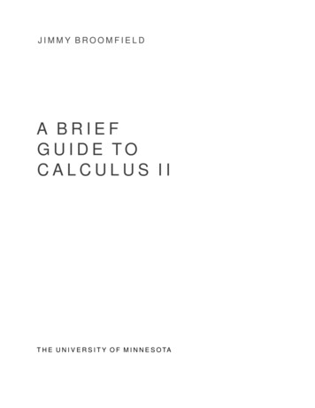
26of f about a horizontal or vertical axis is given byS 2πZ bar(x)q1 [ f 0 ( x )]2 dxwhere r ( x ) is the distance between the graph of f and the axis of revolution.If x g(y) on the interval [c, d], then the surface area isS 2πZ dcr (y)q1 [ g0 ( x )]2 dywhere r (y) is the distance between the graph of g and the axis of revolution.y2Example 1.27. The arc of the parabola y x from x 0 to x 2 isrotated about the y-axis. Find the resulting surface area.4Solution: To begin, notice thatxdy 2x.dx2Rotation of f ( x ) x2 about the y-axis.ThereforeS Z 20 2πs 1 2πxZ 2 p0xdydx 2dx1 4x2 dxNow we will let u 1 4x2 , and thus du 8x dx. Then with the properlimits of integration, we haveS π4Z 17 1u du 17π(2/3)u3/241 π(17 17 1)6Example 1.28. The arc of y cos x from x 0 to x 2π is rotated aboutthe y-axis. Find the resulting surface area.ySolution: To begin, notice thatdy sin xdxRotation of f ( x ) cos x for x [0, 2π ]about the y-axis.
27ThereforeS Z 2π02πxq1 sin2 ( x ) dxFor this example, we concede that the integral above cannot be evaluated analytically by our methods. However if we evaluate this integral numerically,we have the followingS 150.82Example 1.29. (Gabriel’s Horn) For our final example, we will calculatethe surface area of Gabriel’s Horn. This is the surface area of revolution ofy 1/x about the x-axis from x 1 to x .Solution: To begin, notice thatdy 1 2dxxThereforeS Z 1 2π2π f ( x )q1 f 0 ( x )2 dxZ r1x11 1dx.x4Now we will use the comparison test for integrals with the following observationq1 1x4 1on the interval [1, ). Therefore we haveS 2π 2πZ r1x1Z 11xdx 1 1dxx4 This concludes our examples in this section. Make sure to workthrough several examples to see the difficulties and intricacies ofworking surface area problems.Application to Physics and EngineeringIn this section we will consider two applications. The first will beto study fluid pressure and force. The section application will be toconsider the center of mass of a uniform mass distribution.
28Fluid Force and Fluid PressureIn this section we will consider two principles that will help us tocalculate pressure and force on an object submerged in a fluid. Thefirst physical law that we will consider is Pascal’s Principle. Thisstates that the pressure exerted by a fluid on an object at depth d istransmitted equally in all directions.The second principle that we need is that the fluid pressure increases the deeper that an object is submerged. This is seen in thefollowing formulaDefinition 1.30. The pressure on an object at depth d is defined to be theforce per unit are:FP ρgdAwhere ρ is the density of the fluid and g is the acceleration constant due togravity. The constant g is given by g 9.8m/s2 and the density of water isgiven by ρ 1000kg/m3 . Likewise we can solve for pressure to givePA F ρgd.ARemark 1.31. Notice that the principles above allow us to use integration tocalculate the force exerted by a fluid on a vertical plate. This is given in thefollowing definition.Definition 1.32. The force F exerted by a fluid of density ρ on a verticalplane region from y a to y b is given byZ bρgah(y) L(y) dywhere h(y0 ) gives the depth of the fluid at y y0 , and L(y0 ) gives thehorizontal length of the region at height y y0 .Now let us consider an example using this formula.Example 1.33. A trapezoidal plate having the dimensions 8m across on thetop, 6m across on the bottom, and a height of 5m, is submerged in a pool ofwater. Find the force on the plate if it is submerged vertically so that the topis 4m below the surface of the pool.Solution: First we must find formulas for h(y) and L(y). For h(y), we willset the x-axis to sit on the top of the water, and we will center the y-axis tothe center of the trapezoid. This will lead toh(y) y.Next we will notice that L( x ) is given by two times the x coordinate ofan edge of the plate. This can be seen in the diagram on the following page.
29Next, observe that we have L(y) in terms of x. This means that we mustfind a relationship between the x coordinate of the right edge of the plate andy. To do this, we will use the point slope formula to find the equation for theline passing through the points (3, 9) and (4, 4). Therefore we havey 9 5( x 3)and this leads to the following expression for xx y 24.5ThereforeL(y) 2(y 24).5Finally, we must find the limits of integration. These are given by a 9 and b 4. Therefore we have the following calculation
30F ρgZ 4 9 9800 3920h(y) L(y) dyZ 4 9Z 9 4( y) 2(y 24) dy5y2 24y dyy3 3920 12y23 1675 39203 9 4 2.19 106 NFor this section, we have only completed one example, but please checkmoodle for other examples.Moments and Centers of MassIn this next section, we will consider the problem of finding thecenter of mass of a two dimensional plate, and the moment of asystem of masses. We will begin this section by first considering aone dimensional problem.To find the center of mass or balancing point of a one-dimensionalsystem of two point masses of the following systemis given by the following formulax M1 x1 M2 x2M1 M2
31This can be extended to several point masses m1 , ., mn lying alongthe x-axis at positions x1 , ., xn . In this case, we have the followingnx (1/M) mi xii 1nWhere M mi is the total mass of the system and the terms mi xii 1are referred to as moments about the point (0, 0).This can be further extended to a system of masses in two dimensions. Consider a system of n particles with masses m1 , ., mn locatedat the points ( x1 , y1 ), ., ( xn , yn ) in the xy-plane. Following the onedimensional case, we define the moment of the system about they -axis to benMy mi xii 1and the moment of the system about the x -axis isnMx mi yi .i 1Then the center of mass of this system is given by ( x, y) wherex My,my andMx,mnm mii 1Centroid of a LaminaFinally, we will extend our results to find the centroid of a flat plateor lamina in the xy-plane. The following gives us the result that weseekDefinition 1.34. Let f and g be continuous functions such that f ( x ) g( x ) on [ a, b], and consider the lamina of uniform density ρ bounded by thegraphs of y f ( x ) and y g( x ) and a x b.1. The moments about the x -axis and y -axis areMx ρ Z b f ( x ) g( x )2aMy ρZ ba[ f ( x ) g( x )] dxx [ f (
see "Calculus Early Transcendentals", volume I, 7E by James Stewart. To begin this guide, we will review basic integration formula that every calc II student should know, and then move to new techniques. Basic Integrals The integrals below are essential formulas the should be memorized. If you struggle with a few of them, please practice until .