Transcription
108MATHEMATICS MAGAZINEIntegrals Don’t Have Anything to Do withDiscrete Math, Do They?P. MARK KAYLLUniversity of MontanaMissoula, MT 59812-0864mark.kayll@umontana.eduTo students just beginning their study of mathematics, the subject appears to come intwo distinct flavours: continuous and discrete. The former is embodied by the calculus, into which many math majors delve extensively, while the latter has its own introductory course (often entitled Discrete Mathematics) whose overlap with calculusis slight. The distinction persists as we learn more mathematics, since most advancedundergraduate math courses have their focus on one side or the other of this apparentdivide.This article attempts to bridge the divide by describing one surprising connectionbetween continuous and discrete mathematics. Its goal is to convince readers that thetwo worlds are not so very far apart. Though they may frequently feel like polar opposites, there are also times when they join to become one, like antipodal points in projective space. Therefore, any serious study of discrete math ought to include a healthydose of the continuous, and vice versa.Before we are done, various players from both worlds will make their appearance:rook polynomials, derangements, the gamma function, and the Gaussian density (justto name the headliners).Teaser To whet the reader’s appetite, we begin with a challenge.P ROBLEM 1. Give a combinatorial proof thatZ0 (t 3 6t 2 9t 2)e t dt 1;(1)i.e., count something that, on one hand, is easily seen to number the left side of (1) andon the other, the right.For a delightful treatment of combinatorial proofs in general, see [4].At first blush, Problem 1 may appear to be out of reach—a combinatorial proof ofan integral identity—what in heavens should we count? The answer provides part ofthe fun of writing (and hopefully reading) this article.Entities: continuous and discreteAfter introducing our objects of study, we reveal some of their connections in thenext few sections, and also present a solution to Problem 1. In an attempt to make thearticle self-contained, we include an appendix containing some basic facts and othercuriosities about these objects.Math. Mag. 84 (2011) 108–119. doi:10.4169/math.mag.84.2.108. c Mathematical Association of America
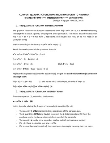
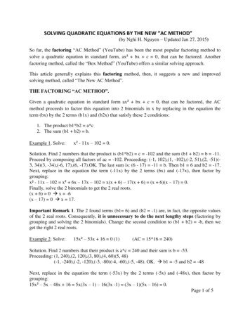
109VOL. 84, NO. 2, APRIL 2011Integrals The integral on the left side of (1) belongs to a family of integrals enjoyingdiscrete connections. The family’s matriarch is Euler’s gamma function, which can bedefined, for 0 x , byZ 0(x) : t x 1 e t dt.(2)0One can check that this improper integral converges for such x; see, e.g., [2, pp. 11–12]. (In fact, 0 need not be confined to the positive real numbers—it is possible toextend its definition so that 0 becomes a meromorphic function on the complex plane,with poles at the origin and each negative integer; see, e.g., [1, p. 199] or [11, p. 54]—but we’ll restrict our attention to positive real x.)Some close cousins of the gamma function are certain ‘probability moments.’ Forintegers n 0, the nth moment (of a Gaussian random variable with mean 0 and variance 1, i.e., a standard normal random variable) is defined byZ 12t n e t /2 dt.Mn : 2π These integrals also converge (see, e.g., [8, p. 148]), and though probability languageenters in their naming, we won’t be making much use of this connection. Since we doneed the fact that M0 1 (see Theorem 4), we present a standard proof of this identityin the Appendix (Lemma 6).Graphs The right side of (1)—i.e., the number 1—counts the ‘perfect matchings’in a certain graph. While we shall assume that the reader is familiar with graphs, wenevertheless introduce the few required elementary notions. Any standard graph theorytext should suffice to close our expositional gaps; see, e.g., [5].Recall that a graph G (V, E) consists of a finite set V (of vertices), togetherwith a set E of unordered pairs {x, y} (edges) with x 6 y and both of x, y V . (Suchgraphs are called simple graphs in [5, p. 3].) A graph is complete if, for each pairx, y of distinct vertices, the edge {x, y} appears in E. F IGURE 1 depicts the completegraphs with 1 V 6 and introduces the standard notation K n for the completegraph on n 1 vertices.K1K2K3Figure 1K4K5K6Complete graphs on up to six verticesThe second graph family of primary interest in this article is the collection of bipartite graphs G, i.e., those for which the vertex set admits a partition V X Y intononempty sets X, Y such that each edge of G is of the form {x, y}, with x X andy Y . One often forms a mental picture of a bipartite graph by imagining two rowsof dots—a row for X and a row for Y —together with a collection of line segments x yjoining an x X to a y Y whenever {x, y} E. In the next definition, we fix twopositive integers n, m. The bipartite graph (X Y, E) for which X n, Y m,and E consists of all nm possible edges between X and Y is called a complete bipartitegraph and denoted by K n,m . The bipartite graphs arising in this article are the complete
110MATHEMATICS MAGAZINEbipartite ones for which n m (for n 1) and their spanning subgraphs, i.e., thosebipartite graphs (X Y, E) with X Y n. It’s worth noting that a subgraph Hof G is a spanning subgraph exactly when they share a common vertex set; the edgeset of H may form any subset of the edge set of G, including the empty set. F IGURE 2depicts a few small bipartite graphs.XY(a) a bipartite graph(b) the complete bipartite graph K3,3Figure 2(c) a spanning subgraph of K3,3Bipartite and complete bipartite graphsA first brush between continuous and discrete For the gamma function (2), it iseasy to check that 0(1) 1, and integration by parts yields the recurrence0(x 1) x0(x),(3)valid for positive real numbers x. It follows by mathematical induction that each nonnegative integer n satisfies 0(n 1) n!; i.e., the gamma function generalizes thefactorial function to the real numbers.Given this generalization, a natural question to ponder might be: What values does0 take on at half-integers? The reader might enjoy showing that 10 π(4)2and then using (3) to prove that 1(2n)! π0 n 24n n!whenever n is a nonnegative integer. (Corollary 7 in the Appendix provides a key stepin this exercise.) The ease in determining 0 at half-integers belies the dearth of knownexact values; for example, no simple expression is known for 0(1/3) or 0(1/4)—see[11, p. 55], or, for a more recent and specific discussion, [15].What good, we might ask, is a continuous version of the factorial function? Oneanswer is that a careful study of 0 can be used to establish Stirling’s approximationfor n!: n n n! 2πn,(5)epublished by James Stirling [18, p. 137] in 1730. (Here and below, the symbol means that the ratio of the left to the right side tends to 1 as n .) See, e.g., [14]for an elementary proof of (5) starting from the definition (2) of 0. A complex-analyticproof, based on the extension of 0 to C r {0, 1, 2, . . .} to which we alluded earlier,appears in [1, pp. 201–204]. However it’s reached, the estimate (5), involving two ofthe most famous mathematical constants and invoking only basic algebraic operations,is no doubt beautiful. Moreover, it is useful any time one wants to gain insight into the
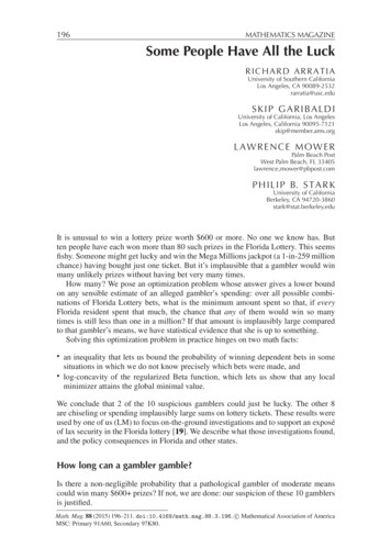
111VOL. 84, NO. 2, APRIL 2011growth rate of functions involving factorials. For example, using (5), one easily showsthat 2n22n ,nπn and so learns something about the asymptotics of the Catalan numbers 2nn /(n 1)(see, e.g., [17, pp. 219–229] for more on this pervasive sequence).Our purpose is to refute the first part of this article’s title, and as we move in thatdirection, we can’t resist sharing a couple more fun facts about 0 that enhance thestature of 0 in the gallery of basic mathematical functions. First, as long as x is not aninteger, we have0(x)0(1 x) π,sin(π x)which generalizes (4). This ‘complement formula’ was first proved by Leonhard Euler;see, e.g., [1, pp. 198–199] or [11, p. 59] for modern proofs. Second, ifζ (x) : X1kxk 1denotes the Riemann zeta function, then whenever 0(x) is finite, we haveZ x 1tζ (x)0(x) dt,et 10(6)which bears a striking resemblance to (2); again, see [1, p. 214] or [11, pp. 59–60] forproofs. Because of ζ ’s central role in connecting number theory to complex analysis,the relation (6) opens deeper connections of 0 to number theory (beyond those stemming from the factorial function). Viewing number theory as falling within the discreterealm, we see in (6) a further refutation of this article’s title.Counting perfect matchings in Kn,nA matching M in a bipartite graph G (X Y, E) is a subset M E such that theedges in M are pairwise disjoint. We think of M as ‘matching up’ some members ofX with some members of Y . If every x X appears in some e M, and likewise forY , then we call M a perfect matching. It is a simple exercise to show that if G containsa perfect matching, then X Y , so that G is a spanning subgraph of some K n,n .F IGURE 3 highlights one matching within each of the graphs in F IGURE 2.(a)(b)(c)Figure 3 Matchings in the graphs of FIGURE 2 indicated by bold edges; those in (b) and(c) are perfect.
112MATHEMATICS MAGAZINEGiven a bipartite graph G, we might be interested to know how many perfect matchings it contains; we use (G) to denote this number.1 Let’s warm up by asking for thevalue of (K n,n ); a moment’s reflection shows that for each integer n 1, the answer is n!. (To see this, continue to denote the ‘bipartition’ by (X, Y ), and notice thatthe perfect matchings of K n,n are in one-to-one correspondence with the bijectionsbetween X and Y .) Since n! 0(n 1), we have proven our first result.Z t n e t dt.P ROPOSITION 2. (K n,n ) 0If we replace K n,n by a different bipartite graph, how must we modify the formulain Proposition 2? It turns out that a so-called ‘rook polynomial’ should replace thepolynomial t n .Rook polynomials Given a graph G and an integer r , we denote by µG (r ) the number of matchings in G containing exactly r edges.E XAMPLE 1. (T HE GRAPH G K 3,3 {{x1 , y1 }, {x2 , y2 }, {x3 , y3 }}) This is thegraph in F IGURE 2(c). Since the empty matching contains no edges, we have µG (0) 1; since each singleton edge forms a matching, we have µG (1) 6, and since G contains two perfect matchings, we have µG (3) 2. Fixing a vertex x, we see that thereare three matchings of size two using either of the edges incident with x and threemore two-edge matchings not meeting x; thus µG (2) 9.Now suppose that G is a spanning subgraph of K n,n . The rook polynomial of G isdefined bynXRG (t) : ( 1)r µG (r )t n r .r 0See [10, p. 8] or [16, pp. 164–166] for the etymology of this term.E XAMPLE 1. ( CONTINUED ) Based on our observations in the first part of this example, we see thatRG (t) t 3 6t 2 9t 2;we’re getting a little ahead of ourselves, but this is the polynomial appearing in theintegrand in Problem 1.E XAMPLE 2. (E MPTY GRAPHS ) If G is the empty graph on 2n vertices (i.e., V 2n and E ), then(0 if r 0µG (r ) 1 if r 0,so that RG (t) t n ; keeping ahead of ourselves, notice that this polynomial appears inthe integrand in Proposition 2.E XAMPLE 3. (P ERFECT MATCHINGS ) If G consists of n pairwise disjoint edges (i.e., G is induced by a perfect matching), then one can easily see that µG (r ) nr for0 r n. Thus, the binomial theorem shows that RG (t) (t 1)n .1 Wechose this notation because (whether we write it in English or Greek!) the letter XI ( ) resembles aperfect matching in a graph of order six, and, conveniently enough, six is a perfect number.
113VOL. 84, NO. 2, APRIL 2011Continuing to let G denote a spanning subgraph of K n,n , we now define its bipartitee this graph shares the vertex set of G and has for edges all the edges ofcomplement G;K n,n that are not in G. We’re ready to state a generalization of Proposition 2. To avoidpossible confusion as to which graph is being complemented, we use next H insteadof G to denote a generic graph.T HEOREM 3. (G ODSIL [9, T HEOREM 3.2]; J ONI AND ROTA [12, C OROLLARY2.1]) If H is a spanning subgraph of K n,n , thenZ (H ) R He(t)e t dt.0The proof of Theorem 3 is beyond our scope, but we’ll present two applications inthe following sections; [7] presents a recent proof. Theorem 3 generalizes Proposition 2 because the bipartite complement of K n,n is the empty graph on 2n vertices; seeExample 2. Further generalizations of Theorem 3 are discussed in [10, pp. 9–10].Solution to Problem 1. As noted in Example 1, the integral in Problem 1 isZ Z 32 tRG (t)e t dt,(t 6t 9t 2)e dt (7)00where, recall, G is the graph depicted in F IGURE 2(c) and defined at the start of Example 1. Thus, to bring Theorem 3 to bear, it will suffice to determine a spanninge G. The graph H in F IGURE 4 does the trick.subgraph H of K 3,3 such that HNow ask: how many perfect matchings are contained in H ? The answer is obviously(H ) 1 because H is induced by the edges of a perfect matching. On the other hand,e G.Theorem 3 tells us that (H ) coincides with (7) because HHe G from FIGURE 2(c)Figure 4 A graph H with HThe fruit borne by the instantiation of Theorem 3 to the graphs in Examples 1 and 2(respectively, a solution to Problem 1 and a proof of Proposition 2) might providee being theinspiration to consider this theorem in yet another instance, this time with Hgraph(s) in Example 3. This application of Theorem 3 takes us down an atypical pathto a commonly studied class of combinatorial objects.Derangements A derangement σ of a set S is a permutation of S with no fixedpoints; i.e., σ : S S is a bijection such that σ (x) 6 x for each x S. Countingthe number of derangements of a finite set is a standard problem in introductorycombinatorics and probability texts. We’ll let Dn denote the set of derangements of{1, 2, . . . , n} and dn Dn . We can easily determine these parameters for the smallestfew values of n; TABLE 1 displays the results. We leave it as an exercise to show thatd5 44 and (for the punishment gluttons) d6 265. But what is the pattern? Perhapssurprisingly, one way to obtain a general expression for dn is to invoke Theorem 3.Consider the bipartite graph G obtained from K n,n by removing the edges of a perfect matching; say, G K n,n {{x1 , y1 }, {x2 , y2 }, . . . , {xn , yn }}. Notice that each perfect matching in G corresponds to exactly one derangement of {1, 2, . . . , n} and vice
114MATHEMATICS MAGAZINETABLE 1: Derangement numbers and their correspondingderangements for 1 n 4ndnDn12340129 {21}{231, 312}{2143, 2341, 2413, 3142, 3412, 3421, 4123, 4312, 4321}versa. Thus, dn (G). Since the bipartite complement of G is the graph consideredin Example 3, Theorem 3 implies thatZ dn (t 1)n e t dt.(8)0If we separate the integral and change variables on the first subinterval, an evaluationof 0 presents itself:Z 1Z n t(t 1)n e t dt(t 1) e dt dn 01Z x n e (x 1) d x 1Z00 e 1 0(n 1)(t 1)n e t dt En ,(9)where we now view the second integral as an error term E n . It turns out that E n doesn’tcontribute much to dn ; since e t 1 on the interval (0, 1), we obtainZ 1Z 11 E n (t 1)n e t dt (1 t)n dt .n 100This shows that for each n 1, the error satisfies E n 1/2, and it follows from (9)that dn is the integer closest to e 1 0(n 1), i.e., to n!/e.Remarks The nonstandard derivation of dn presented above is due to Godsil [10,pp. 8–9]. More typical approaches (e.g., [6, pp. 77–78] or [13, pp. 71, 109–110])—that apply either the principle of inclusion-exclusion or generating functions—lead toa perhaps more familiar expressiondn n!nX( 1)kk 0k!(10)for the derangement numbers. Starting from (8), this ‘standard’ expression (10) for dnrequires even less effort to derive than the former. We first apply the binomial theorem,obtaining!Z Xn nk n kdn ( 1) te t dtk0k 0 n!nXk 0( 1)kk! (n k)!Z0 t n k e t dt,(11)
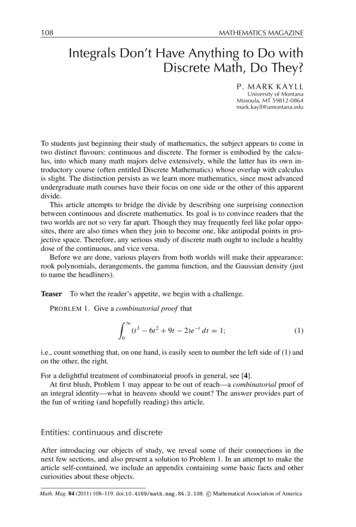
115VOL. 84, NO. 2, APRIL 2011and then invoke the definition (2) of 0 to replace each integral by (n k)!, after which(11) becomes (10). Alternately, via the MacLaurin series for 1/e, (10) is easily seen tobe equivalent to the ‘integer closest to n!/e’ description obtained via Godsil’s derivation.Counting perfect matchings in KnSince matching enumeration is not confined to the realm of bipartite graphs, it is natural to seek analogues of Proposition 2 and Theorem 3 for determining (K n ) and,more generally, (G) for a spanning subgraph G of K n . Here again, we will exposethe speciousness of this article’s title.A matching M in a graph G (V, E) is defined as it is in a bipartite graph, and,as before, if each v V is an end of some e M, then M is called perfect. F IGURE 5displays all of the perfect matchings admitted by K 4 and some of those admitted by K 6 .The bracketed numbers in F IGURE 5(b) indicate how many different perfect matchingsresult under the action of successive rotation by 60 ; in this way, all 15 2 3 6 3 1 perfect matchings of K 6 are obtained.(a)(b)[2][3][6][3][1]Figure 5 (a) All three perfect matchings in K4 ; (b) five of fifteen perfect matchings in K6Following our earlier line of inquiry, we ask how many perfect matchings are contained in K n . Since matchings pair off vertices, the question is interesting only whenn is even; say n 2m for an integer m 1. Let V : V (K 2m ) {1, 2, . . . , 2m}. Todetermine a matching M, it is enough to decide, for each vertex i V , with which vertex i is paired under M. There are (2m 1) choices for pairing with vertex 1. Havingformed this pair, say {1, j}, it remains to decide how to pair the remaining (2m 2)vertices. Selecting one of these, say k, there are (2m 3) choices for pairing with vertex k, namely, any member of V r {1, j, k}. Continuing in this fashion and applyingthe multiplication rule of counting, we find that(0if n is odd(K n ) (12)(2m 1)(2m 3) · · · 5 · 3 · 1 if n 2m for an integer m 1.The last expression, reminiscent of a factorial, is sometimes called a double factorialwhich is defined, for a positive integer n, by n!! : n(n 2)(n 4) · · · (2 or 1)—see,e.g., [20]. This notation shortens (12) to(0if n is odd(K n ) (13)(n 1)!! if n is even.
116MATHEMATICS MAGAZINEWhen n is even (n 2m), we have(K 2m ) (2m 1)!! (2m)!,2m m!(14)which leads to an alternate way to count (K 2m ): think of determining a matchingby permuting the elements of V in a horizontal line (in (2m)! ways) and then simplygrouping the vertices into pairs from left to right. Of course, this over-counts (K 2m )—by a factor of m! since the resulting m matching edges are ordered, and by a factor of2m since each edge itself imposes one of two orders on its ends. After correcting forthe over-counting, we arrive at (14) and thus have a second verification of (12).As a final refutation of our title, we’ll show that (K n ) can also be expressed as anintegral.T HEOREM 4. (G ODSIL [9, T HEOREM 1.2]; A ZOR ET AL . [3, T HEOREM 1])Z 12(K n ) t n e t /2 dt.2π Proof. The right side of the identity is the moment Mn . Since the integrand of eachMn , for odd n, is an odd function, we haveMn 0whenever n is odd.(15)For even n, say n 2m, we apply induction. Since M0 is the area under the curve forthe probability density function of a standard normal random variable, we haveM0 1;(16)the proof of Lemma 6 below verifies this directly.Fix an integer m 1; starting with M2m 2 and integrating by parts yields the recurrenceM2m (2m 1)M2m 2for m 1.(17)NowM2m (2m 1)!! for m 1(18)follows easily from (16) and (17) by induction. Comparing (15) and (18) with (13)shows that Theorem 4 is proved.Just as Proposition 2 generalizes to Theorem 3, so too does Theorem 4 generalize.For a given (not necessarily bipartite) graph G (now with n vertices instead of theearlier 2n in the bipartite setting), the matchings polynomial is defined by PG (t) : Pbn/2crn 2r. To determine (G), we need to replace the factor t n in ther 0 ( 1) µG (r )tintegrand of Theorem 4 by the matchings polynomial of the complementary graph Gof G. We close this section by stating this analogue of Theorem 3 precisely.T HEOREM 5. (G ODSIL [9, T HEOREM 1.2]) If G is a spanning subgraph of K n ,thenZ 12(G) PG (t)e t /2 dt.2π A proof of Theorem 5 may be found in [10, p. 6].
117VOL. 84, NO. 2, APRIL 2011AppendixAfter establishing that the 0th moment M0 1 (which was needed in the proof ofTheorem 4), we indicate how to obtain (4). Evaluating the integral in the definition ofM0 is an enjoyable polar coordinates exercise.Z 2L EMMA 6.e u /2 du 2π. Proof. Denoting the integral by J, we have Z Z2J2 e u /2 du ZZ2π2 /2dv e (u 2 v 2 )/2du dv(19) Z 0e v Z r e r2 /2dr dϑ,(20)0where we used Tonelli’s Theorem to obtain (19) (see, e.g., [21, Theorem 6.10]) anda switch to polar coordinates to reach (20). Since the inner integral here is unity, theresult follows.Perhaps the simplicity of the preceding proof coloured the views of Lord Kelvin(1824–1907), as hinted in the following anecdote from [19, p. 1139]:Once when lecturing he used the word “mathematician,” and then interruptinghimself asked his class: “Do you know what a mathematician is?” Stepping tothe blackboard he wrote upon it:—Z 2e x d x π . Then, putting his finger on what he had written, he turned to his class and said:“A mathematician is one to whom that is as obvious as that twice two makes fouris to you. Liouville was a mathematician.” Then he resumed his lecture.At any rate, now the relation (4) is almost immediate: C OROLLARY 7. 0(1/2) π.R Proof. By definition, 0(1/2) 0 t 1/2 e t dt. On putting t u 2 /2, we find that R 20(1/2) 2 0 e u /2 du, or, since the last integrand is an even function, 0(1/2) R u 2 /22 edu/2. Now Lemma 6 gives the value of this integral to confirm theassertion.Concluding remarksProposition 2 and Theorem 4 present just twoR examples of combinatorially interestingsequences that can be expressed in the form t n dν for some measure ν and space .This topic is considered in detail in [10, Chapter 9].
118MATHEMATICS MAGAZINEWhat is one to make of these connections between integrals and enumeration? Wedon’t claim that integrals provide the preferred lens for viewing these counting problems. For example, nobody would make the case that the integral in Theorem 4 is the‘right way’ to determine (K n ) because the explicit formula (12) provides a directroute. However, perhaps surprisingly, integrals do offer one lens. And this connection between the continuous and the discrete reveals just one of the myriad ways inwhich mathematics intimately links to itself. These links can benefit the mathematicalbranches at either of their ends. The application to counting derangements illustrateshow continuous methods can shed light on a discrete problem, while Problem 1 and itssolution indicate how a discrete viewpoint might yield a fresh approach to an essentially continuous question. This symbiotic relationship between the different branchesof mathematics should inspire students (and their teachers) not to overly specialize. Asin life, it’s better to keep one’s mind as open as possible.Acknowledgments The author drafted this article during a sabbatical at Université de Montréal. Merci à monhôte généreux, Geňa Hahn, et au Département d’informatique et de recherche opérationnelle. Un merci particulier à André Lauzon, qui a apprivoisé mon ordinateur. Thanks also to Karel Stroethoff who pointed me tothe Lord Kelvin connection and whose post-colloquium observation led to an improvement of the derangementsdiscussion.REFERENCES1. L. V. Ahlfors, Complex Analysis, 3rd ed., McGraw-Hill, New York, 1979.2. E. Artin, The Gamma Function, trans. Michael Butler, Holt, Rinehart and Winston, New York, 1964.3. R. Azor, J. Gillis, and J. D. Victor, Combinatorial applications of Hermite polynomials, SIAM J. Math. Anal.13 (1982) 879–890. doi:10.1137/05130624. A. Benjamin and J. Quinn, Proofs that Really Count: The Art of Combinatorial Proof, Mathematical Association of America, Washington, DC, 2003.5. J. A. Bondy and U. S. R. Murty, Graph Theory, Springer, New York, 2008.6. P. J. Cameron, Combinatorics: Topics, Techniques, Algorithms, Cambridge University Press, Cambridge,UK, 1994.7. E. E. Emerson and P. M. Kayll, Another short proof of the Joni-Rota-Godsil integral formula for countingbipartite matchings, Contrib. Discrete Math. 4 (2009) 89–93.8. M. Fisz, Probability Theory and Mathematical Statistics, 3rd ed., trans. R. Bartoszynski, John Wiley, NewYork, 1963.9. C. D. Godsil, Hermite polynomials and a duality relation for matching polynomials, Combinatorica 1 (1981)257–262. doi:10.1007/BF0257933110. C. D. Godsil, Algebraic Combinatorics, Chapman & Hall, New York, 1993.11. J. Havil, Gamma. Exploring Euler’s Constant, Princeton University Press, Princeton, NJ, 2003.12. S. A. Joni and G.-C. Rota, A vector space analog of permutations with restricted position, J. Combin. TheorySer. A 29 (1980) 59–73. doi:10.1016/0097-3165(80)90047-313. J. H. van Lint and R. M. Wilson, A Course in Combinatorics, Cambridge University Press, Cambridge, UK,1992.14. R. Michel, On Stirling’s formula, Amer. Math. Monthly 109 (2002) 388–390. doi:10.2307/269550415. A. Nijenhuis, Short gamma products with simple values, Amer. Math. Monthly 117 (2010) 733–737. doi:10.4169/000298910X51580216. J. Riordan, An Introduction to Combinatorial Analysis, John Wiley, New York, 1958.17. R. P. Stanley, Enumerative Combinatorics, Vol. 2, Cambridge University Press, Cambridge, UK, 1999.18. J. Stirling, Methodus Differentialis: sive Tractatus de Summatione et Interpolatione Serierum Infinitarum,William Bowyer (printer), G. Strahan, London, 1730.19. S. P. Thompson, The Life of William Thomson, Baron Kelvin of Largs, Macmillan, London, 1910.20. E. W. Weisstein, Double factorial, from MathWorld—A Wolfram Web Resource, available at http://mathworld.wolfram.com/DoubleFactorial.html, 1999–2010.21. R. L. Wheeden and A. Zygmund, Measure and Integral: An Introduction to Real Analysis, Marcel Dekker,New York, 1977.Summary To students just beginning their study of mathematics, the discipline appears to come in two distinctflavours: continuous and discrete. This article attempts to bridge the apparent divide by describing a surprisingconnection between these ostensible opposites. Various inhabitants from both worlds make appearances: rook
119VOL. 84, NO. 2, APRIL 2011polynomials, Euler’s gamma function, derangements, and the Gaussian density. Uncloaking combinatorial proofof an integral identity serves as a thread tying these notions together.MARK KAYLL earned mathematics degrees from Simon Fraser University (B.Sc. 1987) and Rutgers University(Ph.D. 1994), then joined the faculty at the University of Montana in Missoula. To date, he has enjoyed sabbaticalsat University of Ljubljana, Slovenia (2001–2002) and Université de Montréal, Canada (2008–2009). In highschool, while playing with a calculator, he noticed that 1.0000001 raised to the ten millionth power is awfullyclose to the mysterious number e and the following year learned that this theorem is already taken. Three decadesdown the road, he still thinks about e occasionally, as exemplified by his contribution here.Letter to the EditorThe sequence discussed in G. Minton’s Note, “Three approaches to a sequence problem,” in the February issue [4] is known as Perrin’s sequence and has a long history.(Perrin’s sequence is defined by x1 0, x2 2, x3 3, and xn xn 2 xn 3 forn 4.) An important question is: Is an integer prime if and only if it satisfies the Perrincondition, n divides xn ? This question was raised by R. Perrin in 1899. A counterexample, now known as a Perrin pseudoprime, was not discovered until 1982: the smallestone is 271441. This is quite remarkable compared to, say, Fermat pseudoprimes withbase 2, for which 341 is the smallest example. Recent work by J. Grantham [3] showsthat there are infinitely many Perrin pseudoprimes. One can run the Perrin recurrencebackward and verify that if p is prime then x p is divisible by p. When the Perrincondition is enhanced by this additional condition, then the first composite that satisfies both congruences, called a symmetric Perrin pseudoprime, is 27664033. For moreinformation, see the references listed below.S TAN WAGONMacalester College, St. Paul, MN 55105wagon@macalester.eduREFERENCES1. W. Adams and D. Shanks, Strong primality tests that are not sufficient, Math. Comp. 39 (1982) 255–300. doi:10.1090/S0025-5718-1982-0658231-92. D. Bressoud and S. Wagon, A Course in Computational Number Theory, New York, Wiley, 2000, exercise8.18.3. J. Grantham, There are infinitely many Perrin pseudoprimes, J. Number Th. 130 (2010) 1117–1128. doi:10.1016/j.jnt.2009.11.0084. G. Minton, Three approaches to a sequence problem, Math. Mag. 84 (2011) 33–37. doi:10.4169/math.mag.84.1.0335. Online Encyclopedia of Integer Sequences, sequence A013998, Unrestricted Perrin pseudoprimes, http://oeis.org/A0139986. Weisstein, Eric W., Perrin pseudoprime, from MathWorld—A Wolfram Web Resource, l7. Wikipedia entry on “Perrin number,” http://en.wikipedia.org/wiki/Perrin numberMath. Mag. 84 (2011) 119. doi:10.4169/math.mag.84.2.119. c Mathematical Association of America
108 MATHEMATICS MAGAZINE Integrals Don't Have Anything to Do with Discrete Math, Do They? P. MARK KAYLL University of Montana Missoula, MT 59812-0864 mark.kayll@umontana.edu To students just beginning their study of mathematics, the subject appears to come in two distinct avo