Transcription
2392IEEE TRANSACTIONS ON INFORMATION THEORY, VOL. 55, NO. 5, MAY 2009Divergence Estimation for MultidimensionalDensities Via k -Nearest-Neighbor DistancesQing Wang, Sanjeev R. Kulkarni, Fellow, IEEE, and Sergio Verdú, Fellow, IEEEAbstract—A new universal estimator of divergence is presented for multidimensional continuous densities based onk -nearest-neighbor (k -NN) distances. Assuming independent andidentically distributed (i.i.d.) samples, the new estimator is provedto be asymptotically unbiased and mean-square consistent. Inexperiments with high-dimensional data, the k -NN approachgenerally exhibits faster convergence than previous algorithms. Itis also shown that the speed of convergence of the k -NN methodcan be further improved by an adaptive choice of k .Index Terms—Divergence, information measure, Kullback–Leibler, nearest-neighbor, partition, random vector, universal estimation.I. INTRODUCTIONA. Universal Estimation of DivergenceSUPPOSEandare probability distributions on. The divergence betweenandis definedas [23](1)when is absolutely continuous with respect to , andotherwise. If the densities ofandwith respect to theLebesgue measure exist, denoted byand, respecfor -almost every such thattively, withand, then(2)The key role of divergence in information theory and large deviations is well known. There has also been a growing interest inapplying divergence to various fields of science and engineeringfor the purpose of gauging distances between distributions. InManuscript received February 20, 2007; revised June 04, 2008. Currentversion published April 22, 2009. This work was supported in part by ARLMURI under Grant DAAD19-00-1-0466, Draper Laboratory under IR&D6002 Grant DL-H-546263, and the National Science Foundation under GrantCCR-0312413. The material in this paper was presented in part at the IEEEInternational Symposium on Information Theory (ISIT), Seattle, WA, July2006.Q. Wang is with the Credit Suisse Group, New York, NY 10010 USA (e-mail:qingwang@princeton.edu).S. R. Kulkarni and S. Verdú are with the Department of Electrical Engineering, Princeton University, Princeton, NJ 08544 USA (e-mail: kulkarni@princeton.edu; verdu@princeton.edu).Communicated by P. L. Bartlett, Associate Editor for Pattern Recognition,Statistical Learning and Inference.Color versions of Figures 1–6 in this paper are available online at http://ieeexplore.ieee.org.Digital Object Identifier 10.1109/TIT.2009.2016060[2], Bhattacharya considers the problem of estimating the shiftandgenerated accordingparameter , given samplesto density functionsand, respectively. The estimate is the minimizer of the divergence betweenand. Divergence also proves to be useful in neuroscience.Johnson et al. [18] employs divergence to quantify the difference between neural response patterns. These techniques arethen applied in assessing neural codes, especially, in analyzingwhich portion of the response is most relevant in stimulus discrimination. In addition, divergence has been used for detectingchanges or testing stationarity in Internet measurements [6],[21], and for classification purposes in speech recognition [30],image registration [15], [29], text/multimedia clustering [11],and in a general classification framework called KLBoosting[26]. Finally, since mutual information is a special case of divergence, divergence estimators can be employed to estimatemutual information. This finds application, for example, in secure wireless communications, where mutual information estimates can approximate secrecy capacity and are useful for evaluating secrecy generation algorithms [40], [41]. In biology andneuroscience, mutual information has been employed in geneclustering [4], [5], [31], [34], neuron classification [32], etc.Despite its wide range of applications, relatively limited workhas been done on the universal estimation of divergence, see[36], [38] and references therein. The traditional approach is touse histograms with equally sized bins to estimate the densiandand substitute the density estimatesandtiesinto (2). In [38], we proposed an estimator based on datadependent partitioning. Instead of estimating the two densitiesseparately, this method estimates the Radon–Nikodym derivausing frequency counts on a statistically equivalenttivepartition of . The estimation bias of this method originatesfrom two sources: finite resolutions and finite sample sizes. Thebasic estimator in [38] can be improved by choosing the numberof partitions adaptively or by correcting the error due to finitesample sizes. Algorithm G (a self-contained description of thisalgorithm is provided in the Appendix) is the most advancedversion which combines these two schemes. Although this algorithm is applicable to estimating divergence for multidimensional data, the computational complexity is exponential inand the estimation accuracy deteriorates quickly as the dimension increases. The intuition is that to attain a fixed accuracy,the required number of samples grows exponentially with thedimension. However, in many applications, e.g., neural coding[37], only moderately large sizes of high-dimensional data areavailable. This motivates us to search for alternative approachesto efficiently estimate divergence for data in . In this paper,we present a new estimator based on -nearest-neighbor ( -NN)0018-9448/ 25.00 2009 IEEE
WANG et al.: DIVERGENCE ESTIMATION FOR MULTIDIMENSIONAL DENSITIES VIA -NEAREST-NEIGHBOR DISTANCESdistances which bypasses the difficulties associated with partitioning in a high-dimensional space. A -nearest-neighbor divergence estimator is introduced in the conference version [39]of this paper.inB. Nearest Neighbor MethodsThe distance fromto its -NN inisOur proposed estimator forSince its inception in 1951 [13], the nearest neighbor methodhas been shown to be a powerful nonparametric technique forclassification [3], [9], density estimation [28], and regressionestimation [8], [22]. In [19], Kozachenko and Leonenko used-NN distances to estimate differential entropyandproved the mean-square consistency of the resulting estimatorfor data of any dimension. Tsybakov and van der Meulen[35] considered a truncated version of the differential entropy-rate ofestimator introduced in [19] and showed itsconvergence for a class of one-dimensional densities withunbounded support and exponentially decreasing tails. Goriaet al. [16] extended the -NN differential entropy estimatorto -NN estimation, where can be any constant. The recentwork [25] considered the estimation of Rényi entropy anddivergence via nearest-neighbor distances. The assumptionsand the corresponding consistency results are different fromthose presented in this work for divergence estimation. In [37]and [20], the differential entropy based on nearest-neighbordistances is applied to estimate mutual information,via(3)Suppose we are to estimate the divergencebetween two continuous densities and . Letandbe independent and identically distributed(i.i.d.) -dimensional samples drawn independently from thedensities and , respectively. Let and be consistent densityestimates. Then, by the law of large numbers(4)will give us a consistent estimate ofprovided that thedensity estimates and satisfy certain consistency conditions.andare obtained through -NNParticulary, ifdensity estimation, should grow with the sample size such thatthe density estimates are guaranteed to be consistent [28]. Incontrast, in this paper, we propose a -NN divergence estimatorthat is consistent for any fixed . The consistency is shown in thesense that both the bias and the variance vanish as the samplesizes increase. These consistency results are motivated by theanalysis of the -NN differential entropy estimator introducedin [19] and the -NN version presented in [16]. However, ouremphasis is on divergence estimation which involves two setsof samples generated from the two underlying distributions.C.andare continuous densities on. Letandbe i.i.d. -dimensionalsamples drawn independently from and , respectively. Letbe the Euclidean distance1 betweenand its -NN1Otherdistance metrics can also be used, for example, p 1, p 6 2.iniswhereis denoted by.(5)To motivate the estimator in (5), denote the -dimensional.open Euclidean ball centered at with radius bySince is a continuous density, the closure ofconalmost surely. The -NN density estitains samplesismate of at(6)where(7)is the volume of the unit ball. Note that the Gamma functionis defined as(8)and satisfies(9)Similarly, the -NN density estimate ofevaluated atis(10)Putting together (4), (6), and (10), we arrive at (5).D. Paper OrganizationDetailed convergence analysis of the divergence estimator in(5) is given in Section II. Section III proposes a generalizedversion of the -NN divergence estimator with a data-dependent choice of and discusses strategies to improve the convergence speed. Experimental results are provided in Section IV.Appendix A describes Algorithm G which serves as a benchmark of comparison in Section IV. The remainder of the Appendix is devoted to the proofs.II. ANALYSISIn this section, we prove that the bias (Theorem 1) and thevariance (Theorem 2) of the -NN divergence estimator (5)vanish as sample sizes increase, provided that certain mildregularity conditions are satisfied.isDefinition 1: A pair of probability density functionscalled “ -regular” if and satisfy the following conditions forsome:(11)-NN Universal Divergence EstimatorSuppose1. The -NN ofis such that2393L-norm distance,(12)(13)(14)
2394IEEE TRANSACTIONS ON INFORMATION THEORY, VOL. 55, NO. 5, MAY 2009Theorem 1: Suppose that the pair of probability density funcis -regular. Then the divergence estimator as showntionsin (5) is asymptotically unbiased, i.e.,Theorem 2 shows that the -NN estimator (5) is mean-squareconsistent. In contrast to our estimators based on partitioningis indepen[38], in this analysis, we assume thatin order to establish mean-square consisdent oftency (Theorem 2) whereas this assumption is not required forshowing the asymptotic unbiasedness (Theorem 1).The proofs of Theorems 3 and 4 follow the same lines as thoseof Theorems 1 and 2 except that we take into account the factthat the value of depends on the given samples.Alternatively, can be identical for various samples but updated as a function of the sample size. As discussed in [7], [33],the choice of trades off bias and variance: a smaller will leadto a lower bias and a higher variance. In most cases, it is easierto further reduce the variance by taking the average of multipleruns of the estimator. If the sample sizes are large enough, wecan select a larger to decrease the variance while still guaranteeing a small bias.Specifically, let us consider the following divergence estimator:Theorem 2: Suppose that the pair of probability density funcis -regular. Thentions(21)(15)(16)III. ADAPTIVE CHOICE OFA. A Generalized -NN Divergence EstimatorIn Section II, is a fixed constant independent of the data.This section presents a generalized -NN estimator where canbe chosen differently at different sample points. The generalized-NN divergence estimator isis the -NN density estimate of andis thewhere-NN density estimate of andare i.i.d. samplesgenerated according to . The following theorem establishes theconsistency of the divergence estimator in (21) provided certainregularity conditions.Theorem 5: Suppose densities and are uniformly continand. Letandbe positive inteuous ongers satisfying(22)(23)Ifand, thenalmost surely(24)B. Bias Reduction(17)whereis the -NN density estimate of ,isthe -NN density estimate of defined in (6) and (10). Comis addedpared to (5), a correction termis the Digamma functionto guarantee consistency, wheredefined by(18)Theorems 3 and 4 show that the divergence estimator (17) isasymptotically consistent.Theorem 3: Suppose that the pair of probability density functionsis -regular. Ifalmost surely for some, then the divergence estimator as shown in (17) isasymptotically unbiased, i.e.,(19)Theorem 4: Suppose that the pair of probability density funcis -regular. Ifalmost surely for sometions, then(20)To improve the accuracy of the divergence estimator (5),we need to reduce the estimation bias at finite sample sizes.One source of bias is the nonuniformity of the distributionnear the vicinity of each sample point. For example, when theunderlying multidimensional distributions are skewed [20],the -NN divergence estimator will tend to overestimate. Totackle this problem, instead of fixing a constant , we fix the) and count hownearest neighbor distance (denoted assamples and samples fall into the ballmanyrespectively, the intuition being that the biases induced by thetwo density estimates can empirically cancel each other. By thegeneralized estimator (17), we could estimate the divergence by(25)(or samples )where (or ) is the number of samplescontained in the ball.: one possibility isThen the problem is how to choose(26)where(27)(28)
WANG et al.: DIVERGENCE ESTIMATION FOR MULTIDIMENSIONAL DENSITIES VIA -NEAREST-NEIGHBOR DISTANCESFig. 1.2395X P Exp(1), Y Q Exp(12), D(P kQ) 1:5682 nats. k 1. In the kernel plug-in method, the divergence is estimated bylog, where the kernel method is used for density estimation.Note that in this casemay not be the exact -NN distancetoor the exact -NN distance fromtofrom. To correct this error, we may keep the distance terms inthe NN estimator and use the divergence estimator in (17) i.e.,TABLE IESTIMATION VARIANCE FORk 1; 2; 4IV. EXPERIMENTS(29)On the other hand, since the skewness of the distributioncauses the problem, we could apply a linear transformation suchthat the covariance matrix of the transformed data is close toidentity matrix. The idea is to calculate the sample covariancematrix based on the datavia(30)where(31)is the sample mean. Then we multiply each centered sample(or) by the inverse of the square root of suchthat the sample covariance matrix of the transformed samples isthe identity matrix. Namely(32)(33)An advantage of the -NN divergence estimators is that theyare more easily generalized and implemented for higher dimensional data than our previous algorithms via data-dependentpartitions [38]. Furthermore, various algorithms [1], [14] havebeen proposed to speed up the -NN search. However, the NNmethod becomes unreliable in a high-dimensional space dueto the sparsity of the data objects. Hinneburg et al. [17] putforward a new notion of NN search, which does not treat alldimensions equally but uses a quality criterion to select relevantdimensions with respect to a given query.The following experiments are performed on simulated datato compare the NN method with Algorithm G (see Appendix)from our previous work using data-dependent partitions [38].Algorithm G combines locally adaptive partitions and finite-sample-size error corrections ([38, Algorithms C and E,respectively]). The figures show the average of 25 independentare equal in the experiments. Fig. 1 showsruns, and anda case with two exponential distributions. The -NN methodexhibits better convergence than Algorithm G as sample sizesincrease. In general, for scalar distributions, Algorithm Gsuffers from relatively higher bias even when a large number ofsamples are available. The -NN method has higher variancefor small sample sizes, but as sample sizes increase, the vari; other choices ofance decreases quickly. Fig. 1 is forgive similar performance in terms of the average of multiple
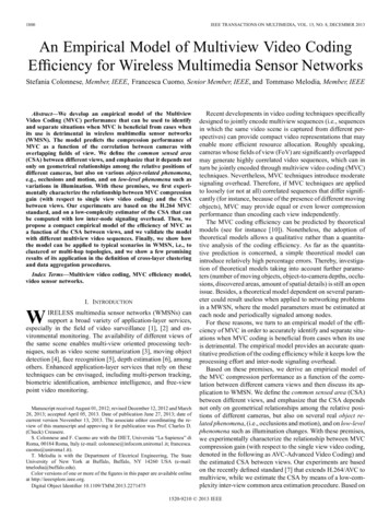
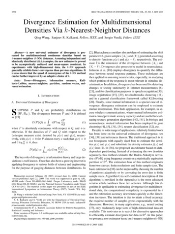
2396IEEE TRANSACTIONS ON INFORMATION THEORY, VOL. 55, NO. 5, MAY 2009C ), Y Q Gaussian( ;CC ); dim 4; [0:1 0:3 0:6 0:9] , [0 0 0 0] , C 1, C 0:5,Fig. 2. X P Gaussian( ;CC 1, C 0:1, for 1; . . . ; 4, s 1; . . . ; 4, 6 s; D(P kQ) 0:9009 nats. k 1.X P Gaussian( ;CC ), Y Q Gaussian( ;CC ); dim 10; 0, C 1, C 0:9, C 1, C 0:1, for 1; . . . ; 10, s 1; . . . ; 10, 6 s; D(P kQ) 6:9990 nats. k 1.Fig. 3.independent estimates. The estimation variance decreases with(see Table I).In Fig. 2, we consider a pair of four-dimensional Gaussiandistributions with different means and different covariance matrices. The -NN estimator converges very quickly to the actualdivergence whereas Algorithm G is biased and exhibits slowerconvergence.In Fig. 3, both distributions are ten-dimensional Gaussianwith equal means but different covariance matrices. The estimates by the -NN method are closer to the true value, whereasAlgorithm G seriously underestimates the divergence. TheIn Fig. 4, we have two identical distributions in-NN method outperforms Algorithm G, which has a very largepositive bias. Note that in the experiments on high-dimensionaldata, the -NN estimator suffers from a larger estimation variance than Algorithm G.In the experiments, we also apply the -NN variants (25) andand , re(29) to the raw data (see curves corresponding tospectively) and we apply the original -NN estimator (5) (with) to the whitening filtered data (33). Results are shown inFigs. 5 and 6. It is observed that the original -NN method withunprocessed data is overestimating and Algorithm G also suf-
WANG et al.: DIVERGENCE ESTIMATION FOR MULTIDIMENSIONAL DENSITIES VIA -NEAREST-NEIGHBOR DISTANCES2397X P Gaussian( ;CC ), Y Q Gaussian( ;CC ); dim 20; 0, C C 1, C C 0:2, for 1; . . . ; 20, s 1; . . . ; 20, 6 s; D(P kQ) 0 nats. k 1.Fig. 4.X P Gaussian( ;CC ), Y Q Gaussian( ;CC ); dim 10; 0, 1, C 1, C 0:999, C 1, C 0:999, 1; . . . ; 10, s 1; . . . ; 10, 6 s; D(P kQ) 0:5005 nats. For each sample point X , (i) is chosen according to (26).Fig. 5.forfers from serious bias. The performance of (25), (29), and thewhitening approach is not quite distinguishable for these examples. All of these approaches can give more accurate results forhighly skewed distributions.In summary, the divergence estimator using the -NN distances is preferable to partitioning-based methods, especiallyfor multidimensional distributions when the number of samplesis limited.APPENDIXA. Algorithm GAlgorithm G is a universal divergence estimator which incorporates two methods from [38].andbe absolutely continuous probability disLet, with.tributions defined onandare i.i.d. samples
2398IEEE TRANSACTIONS ON INFORMATION THEORY, VOL. 55, NO. 5, MAY 2009X P Gaussian( ;CC ), Y Q Gaussian( ;CC ); dim 25; 0, 1, C 1, C 0:9999, C 1, C 0:9999, 1; . . . ; 25, s 1; . . . ; 25, 6 s; D(P kQ) 0:5 nats. For each sample point X , (i) is chosen according to (26).Fig. 6.forgenerated from and , respectively. According to AlgorithmA [38], the divergence is estimated by(34)are the empirical probability measures based onwhere ,is the statistically uniformthe given samples,partition based on-spacing of samples(i.e.,, for all).The estimation bias of (34) can be decomposed into two termsAlgorithm G can be generalized to estimate divergence for. We first partitionintodistributions defined onslabs according to projections onto the first coordinate such thateach slab contains an equal number ofsamples (generatedslabs.from distribution ). Then we scan through all thesamples (generatedFor each slab, if there are many morefrom distribution ) than samples, we further partition thatslab into subsegments according to projections on the second(or ) samples inaxis. Let (or ) denote the number oforblock . We continue this process until(is a parameter) or the partitioning has gone through allthe dimensions of the data. Reduction of finite-sample bias isintegrated in Algorithm G using the approximation (36), wherethe summation is over all the partitions produced by the algorithm.B. Auxiliary Results(35)is due to finite sample sizes, and can be approximated by(36)be aLemma 1: [12, vol. 2, p. 251] Let ,sequence of random variables, which converges in distributionand ato a random variable , and suppose there existsconstantsuch thatfor allis the total number of cells withandwheredenotes that the sum is taken over allwith.is due to finite resolution. The magnitude ofrelieson the partition as well as the underlying distributions and canbe decreased by updating the partition according to the distriby lobutions. In [38], Algorithm C is proposed to reducecally updating the partition according to; Algorithm E compensates for finite sample sizes by subtracting an approximation of . Algorithm G, which combines approaches C and E,achieves better accuracy for various distributions.Then, for all(37)and all integersasLemma 2: Let(38)be a distribution function. Then for(39)
WANG et al.: DIVERGENCE ESTIMATION FOR MULTIDIMENSIONAL DENSITIES VIA -NEAREST-NEIGHBOR DISTANCESProof: First let us assume both integrals are finite. Integrating by parts, we get2399C. Proof of Theorem 1Rewriteas(47)(40).whereThe fact that if one integral diverges so does the other is easyto show. Assume the left side of (39) it converges, thenwhereThus, we have(48)(41)Since(42)we have(43)ThereforeNow it suffices to show that the right-hand side of (48) conas. Using some of the techniquesverges to.in [19] and [16], we proceed to obtainThencan be derived similarly andcan be obtained by the following thesteps.Step 1: Get the conditional distribution ofgivenand the limit of the distribution as.Step 2: Show that the limit of the conditional expectationascan be obtainedusing the limit of the distribution ofconditioned on.using the limit ofStep 3: Calculate the limit ofas.Step 1:be the conditional distribution ofLetgiven. Then, for almost all, for all(49)(44)If the right side of (39) converges, the equality (39) can beproved similarly.Lemma 3: Letbe a distribution function. Then for(50)(45)whereat leastProof: Integrating by parts, we get, (49) is equivalent to the probability that there existpoints inbelonging to, and(51)(46)where.By considering the limit assimilarly as in the proof of Lemma 2, (45) can be obtainedNote that for almost all, as the radius, we have [19], [24], if(52)
2400IEEE TRANSACTIONS ON INFORMATION THEORY, VOL. 55, NO. 5, MAY 2009where represents the Lebesgue measure. Then it can be shownthat, as, then according toSince we already know thatLemma 2, (63) holds, if we have(64)(53)Letbe a random variable with the distribution functionandbe a random variable with the distribu. The corresponding density function oftion functionisfor someand someNow we are to prove (64).posed as.can be decom-(65)(54)Then forBy Lemmas 2 and 3, it is equivalent to consider the followingintegrals:(55)where the last equality is obtained by the change of the variable. To calculate the integral in (55), first note that(56)andwhich leads to(66)due to the property of Gamma function,We estimate the integrals in (66) separately.Note that(57)Now we only need to consider the first integral in (56). By takingthe derivative of (56) with respect to , we obtain(67)thus(58)Recall that the Digamma function satisfiesfor integer(59)Thus(68)(60)whereTherefore, with (57) and (60), we have(61)Step 2:Note that. Hence(69)(62)for any(70)such that(63)(71)
WANG et al.: DIVERGENCE ESTIMATION FOR MULTIDIMENSIONAL DENSITIES VIA -NEAREST-NEIGHBOR DISTANCES2401and(72)(82)(83)(73)(74)(84)The inequality (69) is due to the fact that(75),, and sufficiently largeand (70) holds for. Equation (72) is obtained by change of variable:.,, s.t.The inequality (73) holds because for. Equation (74) is true for some constants.To prove that the integrals in (73) converge, it suffices to showthat(85)wherein (82), the inequality (83) holdsfor sufficiently large , and (84) is obtained by change of vari.ableFinally, we bound(76)By Lemma 3, equivalently we need to show(86)(77)Sincewhich is implied by the fact that(78)(87)and(79)for positive(88)(80)for sufficiently large,Equation (80) holds sinceis -regular and the condition.(14) is satisfied forBy (71) and (74), it follows that(81)Next consider(89)Combining (89), (85) and (81), we have proved (64) and thus,(63) and as a consequence, the desired result (62).
2402IEEE TRANSACTIONS ON INFORMATION THEORY, VOL. 55, NO. 5, MAY 2009Step 3: We need only to show that for(96)(90)Let us first consider the third term on the right-hand side ofthe preceding equation. As in the proof of Theorem 1, for almostallwhich follows from [27, p. 176] and the fact that(91)(92)(97)(93)where (91) is by Fatou’s lemma, (92) follows from (62), and the. Thelast inequality is implied by condition (13)) forproof of (90) is completed.Using the same approach and the conditions (11) and (12) for, if follows thatwhere (97) follows from the change of the integra. Then it can be shown thattion variable. Therefore, the third. Now we need to proveterm in (96) goes to zero asandthat as(98)By (48), (90) and (94), we conclude that(94)For,,, and, we haveD. Proof of Theorem 2By the triangle inequality, we have(99)The following can be proven by similar reasoning as in Theorem 1:(95)(100)Theorem 1 implies that the second term on the right-hand sideof (95) will vanish as ,increase. Thus, it suffices to showas. By the alternativethatexpression (47) forterms ofand,, i.e.,(101)can be written inFor the last term in (99), forhaveis large enoughsufficiently large, we should. Therefore, when
WANG et al.: DIVERGENCE ESTIMATION FOR MULTIDIMENSIONAL DENSITIES VIA -NEAREST-NEIGHBOR DISTANCES, sinceIfwe obtainis -regular, by conditions (11) and (13),(102)Substituting (100)–(102) into (99) and taking derivatives withrespect to and , we can obtain the conditional joint densityand. This joint density givesof2403for someThus,(109), which implies(110)since we already have (90) and (94). Therefore, the last twoterms of (96) are guaranteed to vanish as.(103)E. Proof of Theorem 5Consider the following decomposition of the error:The passing to the limit in (103) can be justified as in Step 2 inthe proof of Theorem 1 by applying the condition (14).Then(104)which can be proved by condition (13) and the argument in (93)The right-hand side of (104) is equal toThus, (98) holds. Therefore, the third and fourth terms of (96). In the same fashion, we can show that thevanish asfirst two terms of (96) also diminish as sample sizes increase.Now let us consider the last two terms in the right side ofandare(96). Since the samplesandassumed to be independent from each other,are independent givenand( can be equal to ). We have(105)where(111)almostBy the Law of Large Numbers, it follows thatsurely. Hence, for, there existssuch thatfor,.By a result from [10, p. 537] and the conditions (22) and (23),andare uniformly stronglyit can be shown thatconsistent, i.e.,(106)(107)IfTherefore, for almost everyciently large, we havealmost surely(112)almost surely(113)in the support of , for suffi-almost surely(114)Now let us considerwhich is equal to. Henceif(108)(115)
2404IEEE TRANSACTIONS ON INFORMATION THEORY, VOL. 55, NO. 5, MAY 2009whereand the first equality is obtained by Taylor’sexpansion and the first inequality is due to the fact (114). Thenbecause of the uniform convergence of , we could findsuch that,for.all , which implies thatsuch thatSimilarly, it can be shown that there existsfor. Therefore, (111) is upper-bounded byif,.REFERENCES[1] J. L. Bentley, “Multidimensional binary search trees used for associative searching,” Commun. ACM, vol. 18, no. 9, pp. 509–517, 1975.[2] P. K. Bhattacharya, “Efficient estimation of a shift parameter fromgrouped data,” Ann. Math. Statist., vol. 38, no. 6, pp. 1770–1787, Dec.1967.[3] T. M. Cover and P. E. Hart, “Nearest neighbor pattern classification,”IEEE Trans. Inf. Theory, vol. IT-13, no. 1, pp. 21–27, Jan. 1967.[4] Z. Dawy, B. Goebel, J. Hagenauer, C. Andreoli, T. Meitinger, and J.C. Mueller, “Gene mapping and marker clustering using Shannon’smutual information,” IEEE/ACM Trans. Comput. Biol. Bioinform., vol.3, no. 1, pp. 47–56, Jan.-Mar. 2006.[5] Z. Dawy, F. M. Gonzaléz, J. Hagenauer, and J. C. Mueller, “Modelingand analysis of gene expression mechanisms: A communication theoryapproach,” in Proc. 2005 IEEE Int. Conf. Communications, Seoul,Korea, May 2005, vol. 2, pp. 815–819.[6] T. Dasu, S. Krishnan, S. Venkatasubramanian, and K. Yi, “An information-theoretic approach to detecting changes in multi-dimensionaldata streams,” in Proc. 38th Symp. Interface of Statistics, ComputingScience, and Applications (Interface ’06), Pasadena, CA, May 2006.[7] L. Devroye, “A course in density estimation,” in Progress in Probability and Statistics. Boston, MA: Birkhäuser, 1987, vol. 14.[8] L. Devroye, L. Györfi, A. Krzyżak, and G. Lugosi, “On the strong universal consistency of nearest neighbor regression function estimates,”Ann. Statist., vol. 22, no. 3, pp. 1371–1385, Sep. 1994.[9] L. Devroye, L. Györfi, and G. Lugosi, A Probablistic Theory of PatternRecognition. New York: Springer, 1996.[10] L. P. Devroye and T. J. Wagner, “The strong uniform consistency ofnearest neighbor density estimates,” Ann. Statist., vol. 5, no. 3, pp.536–540, May 1977.[11] I. S. Dhillon, S. Mallela, and R. Kuma, “A divisive information-theoretic feature clustering algorithm for text classification,” J. Mach.Learning Res., vol. 3, pp. 1265–1287, Mar. 2003.[12] W. Feller, An Introduction to Probability Theory and Its Applications,3rd ed. New York: Wiley, 1970.[13] E. Fix and J. L. Hodges, “Discriminatory Analysis, NonparametricDiscrimination: Consistency Properties,” USAF School of Aviation Medicine, Randolph Field, TX, Tech. Rep. 4, Project Number21-49-004, 1951.[14] K. Fukunaga and P. M. Nerada, “A branch and bound algorithm forcomputing k -nearest neighbors,” IEEE Trans. Comput., vol. C-24, no.7, pp. 750–753, Jul. 1975.[15] J. Goldberger, S. Gordon, and H. Greenspan, “An efficient image similarity measure based on approximations of KL-divergence betweentwo Gaussian mixtures,” in Proc. 9th IEEE Int. Conf. Computer Vision,Nice, France, Oct. 2003, vol. 1, pp. 487–493.[16] M. N. Goria, N. N. Leonenko, V. V. Mergel, and P. L. N. Inverardi, “Anew class of random vector entropy estimators
estimator introduced in [19] and showed its -rate of convergence for a class of one-dimensional densities with unbounded support and exponentially decreasing tails. Goria et al. [16] extended the -NN differential entropy estimator to -NN estimation, where can be any constant. The recent work [25] considered the estimation of Rényi entropy and