Constructing A Human Atrial Fibre Atlas - Springer PDF Free Download

1y ago

26 Views

1 Downloads

3.78 MB

18 Pages

Report/dmca

Download PDF

Transcription

BIOMEDICALENGINEERINGSOCIETYAnnals of Biomedical Engineering, Vol. 49, No. 1, January 2021 (Ó 2020) pp. wOriginal ArticleConstructing a Human Atrial Fibre AtlasCAROLINE H. RONEY ,1 ROKAS BENDIKAS,1 FARHAD PASHAKHANLOO,2CESARE CORRADO,1 EDWARD J. VIGMOND,3,6 ELLIOT R. MCVEIGH,4NATALIA A. TRAYANOVA,5 and STEVEN A. NIEDERER11School of Biomedical Engineering and Imaging Sciences, King’s College London, London, UK; 2Cardiovascular Division,Department of Medicine, Beth Israel Deaconess Medical Center and Harvard Medical School, Boston, USA; 3IHU Liryc,Electrophysiology and Heart Modeling Institute, fondation Bordeaux Université, 33600 Pessac, Bordeaux, France; 4Departmentof Bioengineering, UC San Diego School of Engineering, San Diego, USA; 5Department of Biomedical Engineering, JohnsHopkins University, Baltimore, USA; and 6University of Bordeaux, IMB UMR 5251, 33400 Talence, France(Received 7 November 2019; accepted 27 April 2020; published online 26 May 2020)Communicated by Smadar Cohen.bilayer simulations (0.61 compared to the other correlations,ranging from 0.37 to 0.56). For sinus rhythm simulations,average activation time is robust to ﬁbre ﬁeld direction;however, maximum differences can still be signiﬁcant.Patient speciﬁc ﬁbres are more important for arrhythmiasimulations, particularly in the left atrium. We propose usingthe ﬁbre ﬁeld corresponding to DTMRI dataset 1 for LAsimulations, and the average ﬁbre ﬁeld for RA simulations asthese optimally predicted arrhythmia properties.Abstract—Atrial anisotropy affects electrical propagationpatterns, anchor locations of atrial reentrant drivers, andatrial mechanics. However, patient-speciﬁc atrial ﬁbre ﬁeldsand anisotropy measurements are not currently available,and consequently assigning ﬁbre ﬁelds to atrial models ischallenging. We aimed to construct an atrial ﬁbre atlas froma high-resolution DTMRI dataset that optimally reproduceselectrophysiology simulation predictions corresponding topatient-speciﬁc ﬁbre ﬁelds, and to develop a methodology forautomatically assigning ﬁbres to patient-speciﬁc anatomies.We extended an atrial coordinate system to map thepulmonary veins, vena cava and appendages to standardisedpositions in the coordinate system corresponding to theaverage location across the anatomies. We then expressedeach ﬁbre ﬁeld in this atrial coordinate system and calculatedan average ﬁbre ﬁeld. To assess the effects of ﬁbre ﬁeld onpatient-speciﬁc modelling predictions, we calculated pacedactivation time maps and electrical driver locations duringAF. In total, 756 activation time maps were calculated (7anatomies with 9 ﬁbre maps and 2 pacing locations, for theendocardial, epicardial and bilayer surface models of the LAand RA). Patient-speciﬁc ﬁbre ﬁelds had a relatively smalleffect on average paced activation maps (range of mean localactivation time difference for LA ﬁelds: 2.67–3.60 ms, and forRA ﬁelds: 2.29–3.44 ms), but had a larger effect on maximumLAT differences (range for LA 12.7–16.6%; range for RA11.9–15.0%). A total of 126 phase singularity density mapswere calculated (7 anatomies with 9 ﬁbre maps for the LAand RA bilayer models). The ﬁbre ﬁeld corresponding toanatomy 1 had the highest median PS density map correlation coefﬁcient for LA bilayer simulations (0.44 compared tothe other correlations, ranging from 0.14 to 0.39), while theaverage ﬁbre ﬁeld had the highest correlation for the RAKeywords—Atrial ﬁbres, Anisotropy, Atrial activation,Atrial ﬁbrillation.INTRODUCTIONAtrial myocytes are arranged with a preferentialmyocyte orientation that varies both across the atrialsurface and through the atrial wall.17 The angle of thispreferential myocyte orientation is often referred to asthe ﬁbre orientation. In contrast to the ventricles thathave a regular transmural ﬁbre orientation,15,26 theﬁbres and anatomy in the atria exhibit higher interindividual variability.16,17 Pashakhanloo et al. performed high resolution ex vivo diffusion tensor magnetic resonance imaging of eight human atria todemonstrate that there are features of the atrial anatomy that are consistent across subjects—including theseptopulmonary bundle, the crista terminalis and thepectinate muscle ﬁbres—but the exact location andorientation of atrial bundles varies.29 Atrial ﬁbredirection within the pulmonary veins (PV) and aroundthe junction of the PV with the left atrial body areAddress correspondence to Caroline H. Roney, School ofBiomedical Engineering and Imaging Sciences, King’s College London, London, UK. Electronic mail: 0Ó 2020 The Author(s)

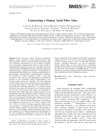
234C. H. RONEY et al.particularly variable between subjects; with reportedﬁbre arrangements including spiralling, circular,chaotic and longitudinal ﬁbres, with either similar ordifferent ﬁbres on the endocardial and epicardial surfaces.16,18,42.Structural anisotropy aﬀects electrical propagationpatterns22 locations of atrial reentrant drivers,34 andatrial mechanics.19 However, current imaging modalities are not suitable for global in vivo measurements ofatrial ﬁbre directions;48 as such it is challenging topersonalise atrial ﬁbre distributions for patient speciﬁcassessment or computational models. There are multiple methodologies for including atrial ﬁbres in either2D surface or 3D volumetric computational meshes.These include rule-based techniques to capture histological descriptions of atrial anatomy and ﬁbre structure.12,20,24,25,44 An alternative approach that may beused to incorporate ﬁbre direction in computationalmodels is to register a ﬁbre atlas to a patient speciﬁcgeometry.20,28,36 Fibre atlases used in current modelling pipelines are either synthetic, constructed in arule-based manner based on histological and morphological descriptions of atrial tissue, or are derivedfrom single large animal datasets.48 These approaches,however, exhibit limited validation, are not representative of individual patients, are not necessarily fromself consistent data sets, and do not always cover bothleft and right atria. In addition, there is growinginterest within the cardiac electrophysiology community in variability, and these deterministic rule-basedmethods do not allow direct propagation of uncertainty through to model simulation output.To address the need for a self consistent data drivenrepresentative ﬁbre map and the correspondinguncertainty quantiﬁcation, we develop a biatrial ﬁbreatlas constructed as an average of the high-resolutionDTMRI dataset of Pashakhanloo et al.29 We ﬁrstproject the ﬁbres for each of the endocardial and epicardial left and right atrial surfaces onto a localcoordinate system. We then construct mean left andright atrial endocardial and epicardial ﬁbre ﬁelds andevaluate the local standard deviation of the ﬁbre orientations. We compare simulated local activation timemaps for each of the meshes with each of the individualﬁbre ﬁelds or the mean ﬁeld. We also simulate atrialﬁbrillation (AF) across the different combinations ofanatomy and ﬁbre ﬁeld and compare arrhythmiaproperties to the patient speciﬁc ﬁbre ﬁeld simulations.Finally, we use the activation time maps and arrhythmia simulation results to determine which of the ﬁbreﬁelds is most representative of the patient-speciﬁc ﬁbreﬁelds, and to propose a ﬁbre atlas for personalisingﬁbres in patient speciﬁc models.BIOMEDICALENGINEERINGSOCIETYMATERIALS AND METHODSWe initially describe the segmentation and meshingsteps used to construct left and right atrial endocardialand epicardial meshes with ﬁbre ﬁelds for each of theex-vivo DTMRI datasets (‘‘Data Modalities’’ and‘‘Segmentation, Meshing and Fibre Assignment’’ sections). We further develop our atrial coordinate systemto ﬁx the locations of the pulmonary veins, vena cavaand appendages at positions in the coordinate systemcorresponding to the average location across the anatomies to minimise the average distortion (‘‘AtrialCoordinates’’ section). We use the atrial coordinatesystem to transfer ﬁbre ﬁelds between atrial geometriesand register all ﬁbres to a single mesh to calculate amean ﬁbre ﬁeld with uncertainty (‘‘Fibre Mapping andCalculating Mean Fibre Fields’’ section), which isvisualised using a streamline based approach (‘‘FibreVisualisation’’ section). Finally we describe themethodologies used for simulating local activationtime maps (‘‘Local Activation Time Simulations’’ section) and arrhythmia simulations (‘‘Arrhythmia Simulations’’ section). The main steps in this methodologyare shown in the schematic in Fig. 1. Data corresponding to the endocardial and epicardial surfacemeshes, their ﬁbre ﬁelds and the average ﬁbre ﬁelds areavailable online (https://doi.org/10.5281/zenodo.3764917 and https://doi.org/10.18742/RDM01-596).Data ModalitiesAll DTMRI data used here are from the study ofPashakhanloo et al. in which human hearts were procured through the National Disease Research Interchange (Philadelphia, PA).29 We used seven out ofeight biatrial datasets from Pashakhanloo et al.29 because for one of the atria we were unable to achieve asegmentation that could be used for calculation of theuniversal atrial coordinates used for registration. Biatrial anatomies were obtained from non-diffusionweighted images (b0), together with DTMRI imagesreconstructed to 0:4 mm 0:4 mm 0:4 mm forassigning ﬁbre ﬁelds to the atrial meshes.Segmentation, Meshing and Fibre AssignmentTo construct an endocardial surface of the left atria,we segmented the blood pool of the b0 images usingour open source segmentation platform, the CEMRGapp (www.cemrgapp.com),39 which was developedusing the medical imaging toolkit (MITK).46 Speciﬁcally, we used the region growing tool on individualslices, together with MITK 3D interpolation. Segmentations were then manually corrected. Right atrialblood pool segmentations required the use of addi-

Constructing a Human Atrial Fibre Atlas(a)235(b)(d)(c)(e)(f)(g)FIGURE 1. Atlas from DTMRI data. (a) MRI data were segmented to give the LA blood pool (red), the LA wall (green), the RA bloodpool (blue) and the RA wall (yellow). (b) The left and right endocardial and epicardial surfaces were meshed. (c) DTMRI fibres wereextracted for each of the LA and RA. (d) Atrial coordinates were calculated (shown here for the LA) and used to express each atriumin a 2D coordinate system. (e) Fibres were expressed in the UAC basis, with a UAC fibre angle. (f) Fibre fields from each of the leftor right atrial endocardial or epicardial shells were registered to a common shell using UAC and an average fibre field wascalculated. (g) Simulations were run to evaluate the effects of fibre field on activation time maps (examples shown here correspondto the fibre fields in (e) and (f).tional tools to accurately segment the detailed pectinate muscle structures. As such, we used 3D regiongrowing with linear thresholding and a connectivityﬁlter of 26-connectivity for each voxel. To outline thepectinate muscle structure, we used a Canny edgedetection ﬁlter. To segment the left or right atrialepicardial surfaces, we initially combined the corresponding endocardial segmentation with the left orright atrial components of the masked image. We thenused an 8-connectivity ﬁlter, together with a cluster sizetolerance of 300 pixels, to ﬁll any holes in the combined segmentation. Speciﬁcally, identiﬁed clustersbounded by the blood pool were categorised as bloodpool, whereas clusters surrounded by mask pixels wereassumed to be holes in the mask. Finally, the segmentation was manually edited using ITK-snap47software to remove any erroneous voxels or ﬁll anymissing areas.Simulation meshes were constructed from thesegmented images using the following sequence ofsteps. First, a marching cubes algorithm implementedwithin the medical image registration toolkit (https://github.com/BioMedIA/MIRTK) was used to extract an isosurface from the segmentation. This surface was then modiﬁed in Meshlab7 using thefollowing sequence of ﬁlters to create a watertightsurface: screened Poisson surface reconstruction,marching cubes, and quadric edge collapse decimation. The resulting surface was then trimmed to openthe mesh at the pulmonary veins (PV), superior venacava (SVC), inferior vena cava (IVC), coronary sinus(CS) and mitral and tricuspid valves (MV and TV)using Paraview software.1 Finally, this mesh was remeshed using mmgtools meshing software (https://github.com/MmgTools/mmg) to produce meshes suitable for simulations, with an average edge length of0.34 mm.Fibres were assigned to each element of these surface meshes by ﬁnding the closest ﬁbre in the DTMRIBIOMEDICALENGINEERINGSOCIETY

236C. H. RONEY et al.ﬁbre ﬁeld to the element mid-point, and projecting thisﬁbre to the surface.Atrial CoordinatesTo register data across atrial anatomies, to create anaverage ﬁbre atlas and to calculate streamlines for ﬁbrevisualisation, each of the left and right atrial endocardial surfaces was expressed in the universal atrialcoordinate (UAC) system.33 UAC were calculatedusing two Laplace solves for each atria with Dirichletboundary conditions of zero and one applied alongtwo sets of boundary nodes. For the LA, the twocoordinates were chosen as a septal to lateral coordinate (aLA ), and a coordinate from the posterior mitralvalve, over the roof, to the anterior mitral valve (bLA ),since these ﬁelds are close to orthogonal and use easilyidentiﬁable atrial structures. Equivalently for the RA,the ﬁrst coordinate passes from the lateral tricuspidvalve to the septal tricuspid valve (aRA ), and the secondcoordinate was from the inferior vena cava to thesuperior vena cava (bRA ).Atrial ﬁbres are inherently deﬁned relative toanatomical structures (the PV, SVC, IVC, CS, left andright atrial appendages). Consequently, mapping ﬁbresbetween cases requires that these structures have thesame UAC values on all meshes. To create a coordinate system with anatomical structures located at thesame UAC, the original UAC system was extended toinclude additional boundary conditions. Detailedmethodology on mapping anatomical structures toatlas coordinate locations, the choice of boundaryconditions and the Laplace solves used to construct theUAC system are given in the supplementary material,and shown in Fig. 2.This implementation uses the VTK and VMTK2python libraries, together with carpentry software forthe Laplace solves (https://carp.medunigraz.at/carputils/). Visualisation was performed using either Paraview1 or meshalyzer software (https://github.com/cardiosolv/meshalyzer).Fibre Mapping and Calculating Mean Fibre FieldsFibres were mapped between atrial anatomies usingthe universal atrial coordinate system. First, UACwere calculated for source and target anatomies asdescribed in the ‘‘Atrial Coordinates’’ section and theSupplementary Material, and as shown in Fig. 3.Local orthonormal bases were constructed using UACfor each element on the source and destinationmeshes.33 The ﬁbre vector ﬁeld on the source mesh wasthen expressed in the UAC basis using barycentricinterpolation. For each element on the destinationmesh, the vector direction in UAC was projected fromBIOMEDICALENGINEERINGSOCIETYthe source geometry to the target geometry in Cartesian space.Fibre angles (h) were expressed in the UAC basis.For the LA, angles were calculated from the aLA axis,so that h 0 (or p) for ﬁbres in the lateral–septaldirection and h p 2 for the posterior–anteriordirection. Figure 3 shows the UAC ﬁbre angles for asource LA mesh mapped to a target LA mesh. For theRA, angles were calculated from the bRA axis, so thath 0 (or p) for ﬁbres in the IVC-SVC direction, andh p 2 for ﬁbres in the lateral–septal direction. Fibrevector ﬁelds are deﬁned between 0 and p since ﬁbrevectors do not have a sense; as such, h values weremapped to fall between 0 and p. We plotted probability density histograms of UAC ﬁbre angle for theLA and RA endocardial and epicardial walls separatedinto the posterior wall region, the roof and the anteriorwall for the LA; or septal, roof and lateral wall for theRA. We split the LA histogram into lateral-septal ﬁbres (h p 4 and h 5p 6) and posterior–anterior ﬁbres (p 4 h 5p 6) and expressed these aspercentages. Similarly, we split the RA histogram intoIVC to SVC ﬁbres (h p 4 and h 5p 6) and ﬁbres inthe lateral–septal direction (from the lateral tricuspidvalve over the roof to the septal tricuspid valve,p 4 h 5p 6). To calculate the mean of the ﬁbrevector ﬁelds, each anatomy and associated ﬁbre ﬁeldwas registered to the same anatomy (following thesteps shown in Fig. 3). We then calculated the circularmean and the circular standard deviation of the ﬁbrevector ﬁeld angles in the range 0 to p, which correctlyaccounts for the discontinuity in angle between 0 and p(implemented using the scipy circmean and circstdfunctions43 with settings low 0, high p to respectﬁbre orientation but disregard ﬁbre direction).Following Krueger,21 we compared the vector ﬁeldsby calculating the angle Ei between two ﬁbre vectorsFi;1 and Fi;2 as: Ei ¼ arccosððFi;1 Fi;2 Þ ðkFi;1 kkFi;2 kÞÞ;where angles greater than p 2 were corrected asEi ¼ p Ei . We then calculated the proportion ofangle differences below p 8, termed Qp 8 21 These differences were calculated separately for the LA posterior wall, roof, anterior wall, LAA and PV, deﬁned asregions in UAC, for the endocardial and epicardialsurfaces. Similarly, for the RA these were calculatedfor the lateral wall, roof, septal wall, RAA and venacavae.Fibre VisualisationTo visualise ﬁbre ﬁelds as streamline trajectories, weadapted the methodology of Saliani et al.38 to workwith the UAC system and the complexity of real ﬁbreﬁelds. As explained in ‘‘Fibre Mapping and Calculat-

Constructing a Human Atrial Fibre Atlas(a)(d)(b)237(c)(e)(f)(g)FIGURE 2. UAC landmarks and paths: (a) 2D points were automatically selected in the original UAC system and mapped to 3D. (b)Geodesic paths or isolines were calculated between the selected 3D points and assigned boundary values, indicated by colour(top: lateral-septal coordinate (aLA ), bottom posterior-anterior coordinate (bLA )). These paths were chosen to fix the location of thePV and LAA as explained in the Supplementary material Section 1.1. (c) These boundary paths are shown in the original UAC (left)and modified UAC (right) system. (d) Laplace solves were performed for the posterior (left) and anterior (right) meshes separatelysubject to the boundary conditions, for the aLA (top) and bLA (bottom) coordinates. (e) The posterior and anterior mesh solutionswere combined to give UAC for the full mesh. (f) Final LA 2D UAC representation. (g) Equivalent steps were used to give the finalRA 2D UAC representationing Mean Fibre Fields’’ section, ﬁbres were expressedin the UAC basis with a UAC ﬁbre angle, h. Streamlines were initially calculated from a random distribution of 10,000 seed points over the atrial surface, andthen a subset of the calculated streamline paths wereselected to generate a streamline ﬁeld with regularspacing and coverage. This calculation is described inthe Supplementary Material.Local Activation Time SimulationsActivation time maps were calculated for each of theleft and right atrial endocardial and epicardial meshesseparately with ﬁbre ﬁelds from each of the anatomies,as well as with the average ﬁbre ﬁeld and with a random ﬁbre ﬁeld to simulate the isotropic case. Equivalent simulations were performed for left and right atrialbilayer models, composed of linearly coupled endocardial and epicardial surfaces with the correspondingﬁbre ﬁelds to those used for the single surface cases.Bilayer meshes were constructed for the LA by duplicating the endocardial surface and projecting 0.1 mmepicardially to generate an epicardial surface, and forthe RA by duplicating the epicardial surface and projecting 0.1 mm endocardially. The projection distanceused here is an arbitrary value that does not representthe atrial wall thickness, which is incorporated in themodel by the choice of coupling coeﬃcient value following Labarthe et al.24 This value can be modiﬁed toreﬂect different coupling between the endocardial andepicardial surfaces due to changes in thickness or thepresence of interstitial ﬁbrosis. Simulations were runusing the carpentry simulator (available at: https://carp.medunigraz.at/carputils/index.html), with a timestep of 20 ls, using the Courtemanche human atrialmodel10 with changes representing electrical remodelling during AF,11,23 together with the monodomainmodel for propagation. To exclude the effects ofrepolarisation heterogeneity, cell model propertieswere either set to left or right atrial properties globally,BIOMEDICALENGINEERINGSOCIETY

238C. H. RONEY et al.FIGURE 3. UAC fibre mapping. An example is shown for mapping LA anatomy 1 with its associated fibre field (the source, toprow) to anatomy 6 (the target, bottom row). Both the source and target anatomies are expressed in UAC (second column). The fibrefield for anatomy 1 is expressed in the UAC basis with UAC angle (h), shown in both 2D and 3D, where h is measured from the aLAaxis. This fibre field is then mapped using UAC to the target anatomy, to give fibre field 1 on anatomy 6 (A6, F1)without modelling any differences in the repolarisationproperties of the pulmonary veins or appendages.Longitudinal conductivity was set to 0.4 S/m andtransverse conductivity to 0.1 S/m.3 Simulations wererun for 1 s of no pacing to reach a steady state, followed by 5 beats at a cycle length of 700 ms; an activation time map was calculated for the ﬁfth beat. Toaccount for conduction anisotropy, activation mapsfor pacing from two separate locations were calculatedfor each anatomy. For the left atrium, pacing was fromthe CS or from the right superior pulmonary vein(RSPV); and for the right atrium, from the right atrialappendage (RAA) or IVC. To ensure anatomies werepaced in equivalent locations, the stimuli locationswere selected manually for the ﬁrst anatomy and thenmapped to the other anatomies using UAC.Spatial ﬁelds of absolute LAT diﬀerences betweensimulations with diﬀerent ﬁbre ﬁelds were calculated andpost-processed to give the median absolute LAT diﬀerence, and maximum absolute LAT diﬀerence expressedas a percentage of the total activation time. The eﬀects ofanisotropy ratio were investigated by modifying the ratiofrom the baseline of 4:1 to 10:1 (longitudinal conductivity0.4S/m, transverse conductivity 0.04S/m).Arrhythmia SimulationsArrhythmias were simulated for left and right atrialbilayer models for each anatomy with ﬁbre ﬁelds fromBIOMEDICALENGINEERINGSOCIETYeach of the anatomies, as well as with the average ﬁbreﬁeld and with a random ﬁbre ﬁeld to simulate theisotropic case. Cell model properties and tissue conductivities were the same as above (‘‘Local ActivationTime Simulations’’ section), with IK1 conductancemodiﬁed to two times the baseline value10 to reduce thewavelength and increase the likelihood that simulatedarrhythmias were sustained.37 To induce AF in each ofthe models using an equivalent set-up, initial conditions corresponding to four spiral wave reentries wereused to automatically generate arrhythmias.27 We usedinitial conditions corresponding to an activation timeﬁeld with two Archimedean spirals on the posteriorwall and two spirals on the anterior wall, with equalUAC spacing between spirals and with opposite chirality for adjacent spirals. Identical initial conditionswere used for the endocardial and epicardial surfaces.For each simulation set-up, phase singularities werecalculated for 10 s of arrhythmia data to identifycentres of rotational activity and re-entrant driverlocations, or until termination if this occurred before10 s. Detected phase singularities were then post-processed to calculated spatial phase singularity densitymaps using our previously published methodology.32We calculated the Pearson correlation coefﬁcientbetween each pair of 2D phase singularity maps usingthe MATLAB corr2 function, where 1 is total positivelinear correlation, 0 is no linear correlation, and 2 1 istotal negative linear correlation.

Constructing a Human Atrial Fibre AtlasRESULTSWe ﬁrst present the left atrial endocardial and epicardial ﬁbre maps coloured by UAC angle (‘‘Left Atrial Fibre Maps’’ section), followed by thecorresponding right atrial maps (‘‘Right Atrial FibreMaps’’ section). We then calculated the average LAand RA ﬁbre ﬁelds across the anatomies by mappingeach anatomy and associated ﬁbre ﬁeld to a single LAand RA anatomy from the dataset using UAC(‘‘Average Fibre Maps’’ section). The effects of ﬁbreﬁeld on local activation time maps during pacing(‘‘Effects of Fibre Field on Local Activation TimeMaps’’ section) and also on electrical reentrant driverlocation during AF (‘‘Effects of Fibre Field onArrhythmia Dynamics’’ section) were determined.Left Atrial Fibre MapsFigure 4 shows endocardial and epicardial ﬁbreﬁelds for seven anatomies, for which streamlines arecoloured by the UAC angle, h. For ﬁbres in the lateralseptal direction, h 0 (or equivalently p, displayed asred or purple); for ﬁbres in the posterior–anteriordirection, h p 2 (green). Visually, six of the sevenanatomies (all except case 3) have posterior–anteriorﬁbres on the roof of the endocardial surface. This isalso evident from the probability density histograms inSupplementary Fig. 1 and Supplementary Sect. 1.2,and the posterior–anterior ﬁbre percentages, which aremoderate except for case 3, which has more ﬁbre vec-239tors in the lateral–septal direction: F1 69.0%, F274.6%, F3 29.3%, F4 58.2%, F5 50.2%, F6 38.8%, F762.8%, FA 59.7%. For the epicardial surface, the roofof anatomies 1, 2, 6 and 7 exhibit ﬁbres in the posterior–anterior direction (posterior–anterior percentages:F1 46.4%, F2 50.5%, F6 52.9%, F7 54.8%), while foranatomies 3, 4 and 5, there is more variability in roofﬁbre direction and lower posterior-anterior ﬁbre percentages (F3 29.8%, F4 39.8%, F5 39.3%, see Supplementary Fig. 2). For each of the anatomies, thereare regions of the posterior wall with ﬁbres orientatedin the lateral-septal direction on both the endocardial(lateral-septal ﬁbre percentages: F1 73:1%, F2 77:8%,F3 88:2%, F4 84:6%, F5 66:6%, F6 51:7%, F7 69:0%,FA 94:8%) and epicardial surfaces (F1 72:4%, F270:6%, F3 81:4%, F4 78:2%, F5 72:0%, F6 72:0%, F765:1%, FA 92:1%). The anterior wall ﬁbres show morevariability between the anatomies, with some showingpredominantly posterior–anterior ﬁbres, some lateral–septal and for some h p 4. This is evident from therange of lateral–septal ﬁbre percentages: F1 70:0%, F250:9%, F3 82:8%, F4 68:5%, F5 73:9%, F6 58:3%, F765:2%, FA 76:7%. Endocardial and epicardial surfacesexhibit regions of similar ﬁbres and also regions withperpendicular ﬁbres at different locations across theanatomies.Right Atrial Fibre MapsFigure 5 shows the corresponding right atrial bodyﬁbre ﬁelds on the endocardial and epicardial surfacesFIGURE 4. Left atrial fibre fields. Left atrial body fibre fields are displayed as streamlines coloured by UAC angle for theendocardial surfaces (top two rows) and epicardial surfaces (bottom two rows). These are shown in posteroanterior view (first andthird row) and anteroposterior view (second and fourth row). Streamlines originating from the PV and LAA are omitted forvisualisation purposes.BIOMEDICALENGINEERINGSOCIETY

240C. H. RONEY et al.FIGURE 5. Right atrial fibre fields. Right atrial body fibre fields are displayed as streamlines coloured by UAC angle for theendocardial (top two rows) and epicardial (bottom two rows) surfaces. These are shown in lateral-septal view (first and third row)and septal-lateral view (second and fourth row). These are orientated such that the IVC-SVC universal atrial coordinate axis isaligned with the x-axis and the lateral-septal coordinate is aligned with the y-axis. UAC angles of 0 or p correspond to the horizontaldirection (aligned with the IVC-SVC coordinate axis), and UAC angles of p 2 correspond to the vertical direction (aligned with thelateral-septal coordinate axis). Streamlines originating from the SVC, IVC, RAA and CS are omitted for visualisation purposes.of the seven anatomies, for which streamlines are coloured by the RA UAC angle, h. Similar to the LAvisualisation, for ﬁbres in the IVC to SVC directionh 0 (or equivalently p, displayed as red or purple);for ﬁbres in the lateral-septal direction (from the lateraltricuspid valve over the roof to the septal tricuspidvalve) h p 2 (green). Several of the anatomies (2, 4, 6and 7) exhibit lateral-septal endocardial ﬁbres runningalong the trabeculated pectinate muscles (see Supplementary Fig. 3 and Supplementary Sect. 1.4). Regionsof the epicardial ﬁbre ﬁeld on the lateral wall are alsoin the lateral-septal direction for each of the anatomies(lateral-septal percentages: F1 42.9%, F2 50.2%, F340.5%, F4 49.7%, F5 71.6%, F6 71.8%, F7 35.5%,FA 55.6%; see Supplementary Fig. 4 and Supplementary Sec. 1.4). The septal wall close to the roofdemonstrates SVC-IVC ﬁbre orientation on both surfaces across the anatomies. Closer to the tricuspidvalve, the septal wall shows more variability in preferential direction between the anatomies.Average Fibre MapsFigure 6 shows average and standard deviation ﬁbreﬁelds for the LA and RA endocardial and epicardialsurfaces. In agreement with the visual assessment in‘‘Left Atrial Fibre Maps’’ section, the average LA ﬁbreﬁelds demonstrate regions of posterior-anterior ﬁbreBIOMEDICALENGINEERINGSOCIETYdirection on the roof (posterior-anterior ﬁbre percentage for LA endocardium: 59.7%; LA epicardium38.9%). For the average LA ﬁbre ﬁeld, a greater proportion of the ﬁbres are orientated in the lateral-septaldirection on the posterior wall than the individual ﬁbreﬁelds: endocardial posterior wall lateral-septal ﬁbrepercentages for the average ﬁeld: 94.8%, compared torange for individual ﬁbre maps: 51.7–88.2%; epicardial: 92.1%, compared to range for individual ﬁ

logical descriptions of atrial anatomy and ﬁbre struc-ture.12,20,24,25,44 An alternative approach that may be used to incorporate ﬁbre direction in computational models is to register a ﬁbre atlas to a patient speciﬁc geometry.20,28,36 Fibre atlases used in current mod-elling pipelines are either synthetic, constructed in a