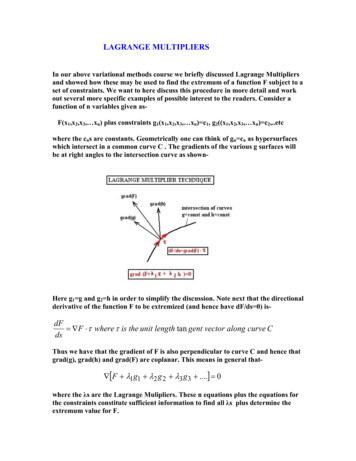
Transcription
Constrained Optimization Using Lagrange MultipliersCEE 201L. Uncertainty, Design, and OptimizationDepartment of Civil and Environmental EngineeringDuke UniversityHenri P. Gavin and Jeffrey T. ScruggsSpring 2020In optimal design problems, values for a set of n design variables, (x1 , x2 , · · · xn ), areto be found that minimize a scalar-valued objective function of the design variables, suchthat a set of m inequality constraints, are satisfied. Constrained optimization problems aregenerally expressed asJ f (x1 , x2 , · · · , xn )minx1 ,x2 ,··· ,xnsuch thatg1 (x1 , x2 , · · · , xn ) 0g2 (x1 , x2 , · · · , xn ) 0.(1)gm (x1 , x2 , · · · , xn ) 0If the objective function is quadratic in the design variables and the constraint equations arelinearly independent, the optimization problem has a unique solution.Consider the simplest constrained minimization problem:minx1 2kx2wherek 0x b.such that(2)This problem has a single design variable, the objective function is quadratic (J 12 kx2 ),there is a single constraint inequality, and it is linear in x (g(x) b x). If g 0, theconstraint equation constrains the optimum and the optimal solution, x , is given by x b.If g 0, the constraint equation does not constrain the optimum and the optimal solutionis given by x 0. Not all optimization problems are so easy; most optimization methodsrequire more advanced methods. The methods of Lagrange multipliers is one such method,and will be applied to this simple problem.Lagrange multiplier methods involve the modification of the objective function throughthe addition of terms that describe the constraints. The objective function J f (x) isaugmented by the constraint equations through a set of non-negative multiplicative Lagrangemultipliers, λj 0. The augmented objective function, JA (x), is a function of the n designvariables and m Lagrange multipliers,JA (x1 , x2 , · · · , xn , λ1 , λ2 , · · · , λm ) f (x1 , x2 , · · · , xn ) mXλj gj (x1 , x2 , · · · , xn )(3)j 1For the problem of equation (2), n 1 and m 1, so11JA (x, λ) kx2 λ (b x) kx2 λx λb22(4)The Lagrange multiplier, λ, serves the purpose of modifying (augmenting) the objectivefunction from one quadratic ( 21 kx2 ) to another quadratic ( 12 kx2 λx λb) so that theminimum of the modified quadratic satisfies the constraint (x b).
2CEE 201L. Uncertainty, Design, and Optimization – Duke – Spring 2020 – Gavin and ScruggsCase 1: b 1If b 1 then the minimum of 12 kx2 is constrained by the inequality x b, and theoptimal value of λ should minimize JA (x, λ) at x b. Figure 1(a) plots JA (x, λ) for a fewnon-negative values of λ and Figure 1(b) plots contours of JA (x, λ).124103.5(a)λ 4(b)augmented cost, JA(x)3Lagrange multiplier, λ83624122.52*1.51b 10.5λ 00-2-1.5-1-0.500.5design variable, x11.502-2-1.5-1-0.500.5design variable, x11.5243.532.5JA21.510.50030.51design variable, x1.5200.513.542.521.5Lagrange multiplier, λFigure 1. JA (x, λ) 21 kx2 λx λb for b 1 and k 2. (x , λ ) (1, 2)CC BY-NC-ND HPG, JTS July 10, 2020
3Constrained Optimization using Lagrange MultipliersFigure 1 shows that: JA (x, λ) is independent of λ at x b, JA (x, λ) is minimized at x b for λ 2, the surface JA (x, λ) is a saddle shape, the point (x , λ ) (1, 2) is a saddle point, JA (x , λ) JA (x , λ ) JA (x, λ ), min JA (x, λ ) max JA (x , λ) JA (x , λ )xλSaddle points have no slope. JA (x, λ) x JA (x, λ) λx x λ λ x x λ λ 0(5a) 0(5b)(5c)For this problem, JA (x, λ) x JA (x, λ) λx x λ λ x x λ λ 0 kx λ 0 λ kx (6a) 0 x b 0 x b(6b)This example has a physical interpretation. The objective function J 12 kx2 representsthe potential energy in a spring. The minimum potential energy in a spring corresponds toa stretch of zero (x 0). The constrained problem:minx1 2kx2such thatx 1means “minimize the potential energy in the spring such that the stretch in the spring isgreater than or equal to 1.” The solution to this problem is to set the stretch in the springequal to the smallest allowable value (x 1). The force applied to the spring in order toachieve this objective is f kx . This force is the Lagrange multiplier for this problem,(λ kx ).The Lagrange multiplier is the force required to enforce the constraint.CC BY-NC-ND HPG, JTS July 10, 2020
4CEE 201L. Uncertainty, Design, and Optimization – Duke – Spring 2020 – Gavin and ScruggsCase 2: b 1If b 1 then the minimum of 21 kx2 is not constrained by the inequality x b. Thederivation above would give x 1, with λ k. The negative value of λ indicatesthat the constraint does not affect the optimal solution, and λ should therefore be set tozero. Setting λ 0, JA (x, λ) is minimized at x 0. Figure 2(a) plots JA (x, λ) for a fewnegative values of λ and Figure 2(b) plots contours of JA (x, λ).12010*-0.5(a)(b)λ -4augmented cost, JA(x)-1Lagrange multiplier, λ8-36-242-1b -1-1.5-2-2.5-3-3.5λ 00-2-1.5-1-0.500.5design variable, x11.5-42-2-1.5-1-0.500.5design variable, x11.5243.532.5JA21.510.50-2-1-1.5-1design variable, x-0.50 -4-3.5-3-0.50-1.5-2-2.5Lagrange multiplier, λFigure 2. JA (x, λ) 21 kx2 λx λb for b 1 and k 2. (x , λ ) (0, 0)CC BY-NC-ND HPG, JTS July 10, 2020
5Constrained Optimization using Lagrange MultipliersFigure 2 shows that: JA (x, λ) is independent of λ at x b, the saddle point of JA (x, λ) occurs at a negative value of λ, so JA / λ 6 0 for anyλ 0. The constraint x 1 does not affect the solution, and is called a non-binding or aninactive constraint. The Lagrange multipliers associated with non-binding inequality constraints are negative. If a Lagrange multiplier corresponding to an inequality constraint has a negative valueat the saddle point, it is set to zero, thereby removing the inactive constraint from thecalculation of the augmented objective function.SummaryIn summary, if the inequality g(x) 0 constrains the minimum of f (x) then theoptimum point of the augmented objective JA (x, λ) f (x) λg(x) is minimized with respectto x and maximized with respect to λ. The optimization problem of equation (1) may bewritten in terms of the augmented objective function (equation (3)),maxminλ1 ,λ2 ,··· ,λm x1 ,x2 ,··· ,xnJA (x1 , x2 , · · · , xn , λ1 , λ2 , · · · , λm )such thatλj 0 j (7)The necessary conditions for optimality are: JA xk JA λk 0(8a) 0(8b)λj 0(8c)xi x iλj λ jxi x iλj λ jThese equations define the relations used to derive expressions for, or compute values of, theoptimal design variables x i . Lagrange multipliers for inequality constraints, gj (x1 , · · · , xn ) 0,are non-negative. If an inequality gj (x1 , · · · , xn ) 0 constrains the optimum point, the corresponding Lagrange multiplier, λj , is positive. If an inequality gj (x1 , · · · , xn ) 0 does notconstrain the optimum point, the corresponding Lagrange multiplier, λj , is set to zero.CC BY-NC-ND HPG, JTS July 10, 2020
6CEE 201L. Uncertainty, Design, and Optimization – Duke – Spring 2020 – Gavin and ScruggsSensitivity to Changes in the Constraints and Redundant ConstraintsOnce a constrained optimization problem has been solved, it is sometimes useful toconsider how changes in each constraint would affect the optimized cost. If the minimumof f (x) (where x (x1 , · · · , xn )) is constrained by the inequality gj (x) 0, then at theoptimum point x , gj (x ) 0 and λ j 0. Likewise, if another constraint gk (x ) does notconstrain the minimum, then gk (x ) 0 and λ k 0. A small change in the j-th constraint,from gj to gj δgj , changes the constrained objective function from f (x ) to f (x ) λ j δgj .However, since the k-th constraint gk (x ) does not affect the solution, neither will a smallchange to gk , λ k 0. In other words, a small change in the j-th constraint, δgj , correspondsto a proportional change in the optimized cost, δf (x ), and the constant of proportionalityis the Lagrange multiplier of the optimized solution, λ j .δf (x ) mXλ j δgj(9)j 1The value of the Lagrange multiplier is the sensitivity of the constrained objective to (small)changes in the constraint δg. If λj 0 then the inequality gj (x) 0 constrains the optimumpoint and a small increase of the constraint gj (x ) increases the cost. If λj 0 thengj (x ) 0 and does not constrain the solution. A small change of this constraint shouldnot affect the cost. So if a Lagrange multiplier associated with an inequality constraintgj (x ) 0 is computed as a negative value, it is subsequently set to zero. Such constraintsare called non-binding or inactive constraints.f(x)f(x)δ f λδgλ 0λ 00111xx*not okokg(x) 00111000111000111not okλ 0 δ f 0okxx*g(x) δgg(x)Figure 3. Left: The optimum point is constrained by the condition g(x ) 0. A small increaseof the constraint from g to g δg increases the cost from f (x ) to f (x ) λδg. (λ 0) Right:The constraint is negative at the minimum of f (x), so the optimum point is not constrainedby the condition g(x ) 0. A small increase of the constraint function from g to g δg doesnot affect the optimum solution. If this constraint were an equality constraint, g(x) 0, thenthe Lagrange multiplier would be negative and an increase of the constraint would decrease thecost from f to f λδg (λ 0).The previous examples consider the minimization of a simple quadratic with a singleinequality constraint. By expanding this example to two inequality constraints we can seeagain how Lagrange multipliers indicate whether or not the associated constraint boundsCC BY-NC-ND HPG, JTS July 10, 2020
7Constrained Optimization using Lagrange Multipliersthe optimal solution. Consider the minimization problemminx1 2kx2such thatx bx cwherek 0and0 b 1000111not xb x* cokFigure 4. Minimization of f (x) 12 kx2 such that x b and x c with 0 b c. Feasiblesolutions for x are greater-or-equal than both b and c.Proceeding with the method of Lagrange multipliers1JA (x1 λ1 , λ2 ) kx2 λ1 (b x) λ2 (c x)(11)2Where the constraints (b x) and (c x) are satisfied if they are negative-valued. Thederivatives of the augmented objective function are JA (x, λ1 , λ2 ) x JA (x, λ1 , λ2 ) λ1 JA (x, λ1 , λ2 ) λ2x x λ1 λ 1λ2 λ 2x x λ1 λ 1λ2 λ 2x x λ1 λ 1λ2 λ 2 0 kx λ 1 λ 2 0(12a) 0 x b 0(12b) 0 x c 0(12c)These three equations are linear in x , λ 1 , and λ 2 .k 1 1x 0 00 λ1 b 1 100λ 2 c (13)Clearly, if b 6 c then x can not equal both b and c, and equations (12b) and (12c) cannot both be satisfied. In such cases, we proceed by selecting a subset of the constraints,and evaluating the resulting solutions. So doing, the solution x b minimizes 21 kx2 suchthat x b with a Lagrange multiplier λ1 kb. But x b does not satisfy the inequalityx c. The solution x c minimizes 21 kx2 . such that both inequalities hold and withwith a Lagrange multiplier λ2 kc. Note that for this quadratic objective, the constraintwith the larger Lagrange multiplier is the active constraint and that the other constraint isnon-binding.CC BY-NC-ND HPG, JTS July 10, 2020
8CEE 201L. Uncertainty, Design, and Optimization – Duke – Spring 2020 – Gavin and ScruggsMultivariable Quadratic ProgrammingQuadratic optimization problems with a single design variable and a single linear inequality constraint are easy enough. In problems with many design variables (n 1) andmany inequality constraints (m 1), determining which inequality constraints are enforcedat the optimum point can be difficult. Numerical methods used in solving such problemsinvolve iterative trial-and-error approaches to find the set of “active” inequality constraints.Consider a third example with n 2 and m 2:min x21 0.5x1 3x1 x2 5x22x1 ,x2such thatg1 3x1 2x2 2 0g2 15x1 3x2 1 0(14)This example also has a quadratic objective function and inequality constraints that arelinear in the design variables. Contours of the objective function and the two inequalityconstraints are plotted in Figure 5. The feasible region of these two inequality constraints isto the left of the lines in the figure and are labeled as “g1 ok” and “g2 ok”. This figure showsthat the inequality g1 (x1 , x2 ) constrains the solution and the inequality g2 (x1 , x2 ) does not.This is visible in Figure 5 with n 2, but for more complicated problems it may not beimmediately clear which inequality constraints are “active.”Using the method of Lagrange multipliers, the augmented objective function isJA (x1 , x2 , λ1 , λ2 ) x21 0.5x1 3x1 x2 5x22 λ1 (3x1 2x2 2) λ2 (15x1 3x2 1) (15)Unlike the first examples with n 1 and m 1, we cannot plot contours of JA (x1 , x2 , λ1 , λ2 )since this would be a plot in four-dimensional space. Nonetheless, the same optimalityconditions hold.min JA x1min JA x2max JA λ1max JA λ2 JA x1 JA x2 JA λ1 JA λ2 0 2x 1 0.5 3x 2 3λ 1 15λ 2 0(16a)x 1 ,x 2 ,λ 1 ,λ 2 0 3x 1 10x 2 2λ 1 3λ 2 0(16b) 0 3x 1 2x 2 2 0(16c) 0 15x 1 3x 2 1 0(16d)x 1 ,x 2 ,λ 1 ,λ 2x 1 ,x 2 ,λ 1 ,λ 2x 1 ,x 2 ,λ 1 ,λ 2If the objective function is quadratic in the design variables and the constraints are linearin the design variables, the optimality conditions are simply a set of linear equations in thedesign variables and the Lagrange multipliers. In this example the optimality conditions areexpressed as four linear equations with four unknowns. In general we may not know whichinequality constraints are active. If there are only a few constraint equations it’s not toohard to try all combinations of any number of constraints, fixing the Lagrange multipliersfor the other inequality constraints equal to zero.CC BY-NC-ND HPG, JTS July 10, 2020
9Constrained Optimization using Lagrange MultipliersLet’s try this now! First, let’s find the unconstrained minimum by assuming neither constraint g1 (x1 , x2 )or g2 (x1 , x2 ) is active, λ 1 0, λ 2 0, and"2 33 10#"x 1x 2#" 0.50#" x 1x 2#" 0.450.14#(17),which is the unconstrained minimum shown in Figure 5 as a “ ”. Plugging this solution into the constraint equations gives g1 (x 1 , x 2 ) 0.93 and g2 (x 1 , x 2 ) 8.17,so the unconstrained minimum is not feasible with respect to constraint g1 , sinceg1 ( 0.45, 0.14) 0. Next, assuming both constraints g1 (x1 , x2 ) and g2 (x1 , x2 ) are active, optimal values forx 1 , x 2 , λ 1 , and λ 2 are sought, and all four equations must be solved together. 233 103215 3x 13 15 2 3 x 2 00 λ 1λ 200 0.50 21 x 1x 2λ 1λ 2 0.10 0.853.55 0.56 ,(18)which is the constrained minimum shown in Figure 5 as a “o” at the intersection of theg1 line with the g2 line in Figure 5. Note that λ 2 0 indicating that constraint g2 is notactive; g2 ( 0.10, 0.85) 0 (ok). Enforcing the constraint g2 needlessly compromisesthe optimality of this solution. So, while this solution is feasible (both g1 and g2evaluate to zero), the solution could be improved by letting go of the g2 constraint andmoving along the g1 line. So, assuming only constraint g1 is active, g2 is not active, λ 2 0, and 0.52 3 3x 1 3 10 2 x2 0 2λ 13 2 0 0.81x 1 x2 0.21 ,0.16λ 1 (19)which is the constrained minimum as a “o” on the g1 line in Figure 5. Note that λ 1 0,which indicates that this constraint is active. Plugging x 1 and x 2 into g2 (x1 , x2 ) gives avalue of -13.78, so this constrained minimum is feasible with respect to both constraints.This is the solution we’re looking for. As a final check, assuming only constraint g2 is active, g1 is not active, λ 1 0, and23 15x 1 0.5 3 10 3 x2 0 15 30λ 21 x 10.06 x2 0.03 ,λ 2 0.04 (20)which is the constrained minimum shown in as a “o” on the g2 line in Figure 5. Notethat λ 2 0, which indicates that this constraint is not active, contradicting our assumption. Further, plugging x 1 and x 2 into g1 (x1 , x2 ) gives a value of 2.24, so thisconstrained minimum is not feasible with respect to g1 , since g1 (0.06, 0.03) 0.CC BY-NC-ND HPG, JTS July 10, 2020
10CEE 201L. Uncertainty, Design, and Optimization – Duke – Spring 2020 – Gavin and Scruggs1(a)0.5x2g1 ok0g2 ok-0.5-1-1-0.50x10.511(b)0.5x2g1 ok0g2 ok-0.5-1-1-0.50x10.51Figure 5. Contours of the objective function and the constraint equations for the example ofequation (14). (a): J f (x1 , x2 ); (b): JA f (x1 , x2 ) λ 1 g1 (x1 , x2 ). Note that the thecontours of JA are shifted so that the minimum of JA is at the optimal point along the g1 line.CC BY-NC-ND HPG, JTS July 10, 2020
11Constrained Optimization using Lagrange MultipliersMatrix Relations for the Minimum of a Quadratic with Equality ConstraintsThe previous example of the minimization of a quadratic in x1 and x2 , subject to twoin linear equality constraints equations (14), may be written, generally as11min H11 x21 H12 x1 x2 H22 x22 c1 x1 c2 x2 d22A11 x1 A12 x2 b1 0A21 x1 A22 x2 b2 0(21)such thatx1 ,x2or, even more generally, for any number (n) of design variables, as minx1 ,x2 ,··· ,xn n XnXnXPnj 1 A1j xjPn b1 0Ax b2 0j 1 2j j. 1xi Hij xj ci x i d 2 i 1 j 1i 1such thatPnj 1(22)Amj xj bm 0P Pwhere Hij Hji and i j xi Hij xj 0 for any set of design variables. In matrix-vectornotation, equation (22) is written1 Tx Hx cT x d2minxAx b 0such that(23)The augmented optimization problem ismaxminλ1 ,··· ,λm x1 ,··· ,xn nmnnn XXXX1X λk Akj xj bk ,ci x i d xi Hij xj 2 i 1 j 1j 1i 1k 1(24)such that λk 0. Or, in matrix-vector notation, max minλx1 Tx Hx cT x d λT (Ax b)2 λ 0.such that(25)Assuming all constraints are “active” the necessary conditions for optimality are JA (x, λ) 0T xand JA (x, λ) 0T λ(26)Ax b 0(27)Which, for this very general system result inHx c AT λ 0andThese equations can be written compactly as a single matrix equation"H ATA 0#"xλ#" cb#(28)Equation (28) is called the Karush Kuhn Tucker (KKT) equation.Comparing equation (14) to equation (22) and comparing equations (18), (19), and(20) to equation (28), you may begin to convince yourself that the KKT system gives ageneral solution for the minimum of a quadratic with linear equality constraints. It is veryuseful.CC BY-NC-ND HPG, JTS July 10, 2020
12CEE 201L. Uncertainty, Design, and Optimization – Duke – Spring 2020 – Gavin and ScruggsPrimal and DualIf it is possible to solve for the design variables x in terms of the Lagrange multipliersλ, then the design variables can be eliminated from the problem and the optimization issimply a maximization over the set of Lagrange multipliers.For this kind of problem, the condition JA (x, λ) 0T x(29)results in Hx c AT λ 0 from which the design variables x may be solved in terms ofλx H 1 (AT λ c).(30)Substituting this solution for x in terms of λ into (25) eliminates x from equation (25) andresults in a really long expression for the augmented objective in terms of λ onlymaxλ 12TT (λ A c )H 1 H H 1T T(A λ c) c H 1T(A λ c) d λT A H 1T(A λ c) b. and after a little algebra involving some convenient cancellations and combinations . we obtainthe dual problem.11max λT AH 1 AT λ (cT H 1 AT bT )λ cT H 1 c dλ22 such that λ 0 (31)Equation (25) is called the primal quadratic programming problem and equation (31)is called the dual quadratic programming problem. The primal problem has n m unknownvariables (x and λ) whereas the dual problem has only m unknown variables (λ) and istherefore easier to solve.Note that if quadratic term in the primal form (quadratic in the primal variable x)is positive, then the quadratic term in the dual form (quadratic in the dual variable λ) isnegative. So, again, it makes sense to minimize over the primal variable x and to maximizeover the dual variable λ.CC BY-NC-ND HPG, JTS July 10, 2020
13Constrained Optimization using Lagrange MultipliersAn Active Set Algorithm for Quadratic ProgrammingAs was shown in the numerical example, in problems with multiple inequality constraints it is often hard to know which of the inequality constraints are active. A trialand-error approach may be attempted to find the set of active inequality constriants, forwhich all the Lagrange multipliers are positive-valued. Anticipating nonlinear problems, wewill assume we know that x is a good but potentially infeasible solution to the quadraticprogram. We wish to update x to a better solution by adding the update vector h, so thatx h solves the quadratic program. To find the “optimal” update vector, we can expressthe quadratic in terms of the known current parameter values x and the unknown updatevector h , 1TTTs.t. λ 0 (32)max min (x h) H(x h) c (x h) d λ (A(x h) b)λh2Expanding equation (32) and deriving the necessary conditions for optimality of the step h, JA (h, λ) 0T hand JA (h, λ) 0T λ(33)A(x h) b 0(34)leads toH(x h) c AT λ 0andwhich may be writtin in a KKT form"H ATA 0#"hλ#" Hx c Ax b#(35)But the question remains, “Which constraint equations are active?” In the following theconstraint equations in the active set are denotedA a x ba 0(36)with Lagrange multipliers λa associated with the constraint equations in the active set.In this active set algorithm, we may start by assuming no constraints are active, so that(0)A(0)a A and ba b.1. In iteration (k), solve"H A(k)aA(k)0aT#"hλ(k)a#" Hx c(k) A(k)a x ba#for h and λ(k)a .2. Evaluate the full set of constraint equations g A(x h) b.3. In Aa(k 1) and b(k 1) include the rows of A and b corresponding to the rows of g thatare positive.4. In Aa(k 1) and b(k 1) exclude the rows of A and b corresponding to the rows of λ(k)athat are negative.5. Assign elements of λ(k)a to the active indices of λ.6. set k k 1 and return to step 1.CC BY-NC-ND HPG, JTS July 10, 2020
4 CEE 201L. Uncertainty, Design, and Optimization - Duke - Spring 2020 - Gavin and Scruggs Case 2: b 1 If b 1 then the minimum of 1 2 kx2 is not constrained by the inequality x b.The derivation above would give x 1, with λ k.The negative value of λ indicates that the constraint does not affect the optimal solution, and λ should therefore be set to