Transcription
TABLES AND FORMULAS FOR MOOREBasic Practice of StatisticsExploring Data: Distributions Look for overall pattern (shape, center, spread)and deviations (outliers). Mean (use a calculator):x 1!x1 x2 · · · xn nnxi Standard deviation (use a calculator):s "1 !(xi x)2n 1 Median: Arrange all observations from smallestto largest. The median M is located (n 1)/2observations from the beginning of this list. Quartiles: The first quartile Q1 is the median ofthe observations whose position in the orderedlist is to the left of the location of the overallmedian. The third quartile Q3 is the median ofthe observations to the right of the location ofthe overall median. Correlation (use a calculator):1 ! xi xr n 1sx# %yi ysy& Least-squares regression line (use a calculator):ŷ a bx with slope b rsy /sx and intercepta y bx Residuals:residual observed y predicted y y ŷProducing Data Simple random sample: Choose an SRS bygiving every individual in the population anumerical label and using Table B of randomdigits to choose the sample. Randomized comparative experiments:"!Random !Allocation# #Group 1 % Treatment 1Group 2 % Treatment 2# Observe#" Response!! Five-number summary:Minimum, Q1 , M, Q3 , Maximum Standardized value of x:x µz σProbability and SamplingDistributions Probability rules: Any probability satisfies 0 P (A) 1. The sample space S has probabilityP (S) 1.Exploring Data: Relationships Look for overall pattern (form, direction,strength) and deviations (outliers, influentialobservations). If events A and B are disjoint, P (A or B) P (A) P (B). For any event A, P (A does not occur) 1 P (A)
Sampling distribution of a sample mean: x has mean µ and standard deviation σ/ n. Two-sample t test statistic for H0 : µ1 µ2(independent SRSs from Normal populations):x1 x2t "s21s2 2n1 n2 x has a Normal distribution if the population distribution is Normal. Central limit theorem: x is approximatelyNormal when n is large.Basics of Inference z confidence interval for a population mean(σ known, SRS from Normal population):σz from N (0, 1)x z n Sample size for desired margin of error m:n #z σm 2x µ0 σ/ nP -values from N (0, 1)Inference About Means t confidence interval for a population mean (SRSfrom Normal population):st from t(n 1)x t n t test statistic for H0 : µ µ0 (SRS from Normalpopulation):t x µ0 s/ nP -values from t(n 1) Matched pairs: To compare the responses to thetwo treatments, apply the one-sample t procedures to the observed differences. Two-sample t confidence interval for µ1 µ2 (independent SRSs from Normal populations):(x1 x2 ) t "s21n1Inference About Proportions Sampling distribution of a sample proportion:when the population and the sample size areboth large and p is not close to 0 or 1, p̂ is approximately' Normal with mean p and standarddeviation p(1 p)/n. Large-sample z confidence interval for p: z test statistic for H0 : µ µ0 (σ known, SRSfrom Normal population):z with conservative P -values from t with df thesmaller of n1 1 and n2 1 (or use software). s22n2with conservative t from t with df the smallerof n1 1 and n2 1 (or use software).p̂ z "p̂(1 p̂)nz from N (0, 1)Plus four to greatly improve accuracy: use thesame formula after adding 2 successes and twofailures to the data. z test statistic for H0 : p p0 (large SRS):z "p̂ p0P -values from N (0, 1)p0 (1 p0 )n Sample size for desired margin of error m:n #z m 2p (1 p )where p is a guessed value for p or p 0.5. Large-sample z confidence interval for p1 p2 :(p̂1 p̂2 ) z SEz from N (0, 1)where the standard error of p̂1 p̂2 isSE "p̂1 (1 p̂1 ) p̂2 (1 p̂2 ) n1n2Plus four to greatly improve accuracy: use thesame formulas after adding one success and onefailure to each sample.
Two-sample z test statistic for H0 : p1 p2(large independent SRSs):z "p̂1 p̂2p̂(1 p̂)#11 n1 n2 where p̂ is the pooled proportion of successes.The Chi-Square Test Expected count for a cell in a two-way table:row total column totalexpected count table total Chi-square test statistic for testing whether therow and column variables in an r c table areunrelated (expected cell counts not too small):X2 ! (observed count expected count)2 t confidence interval for regression slope β:b t SEbt from t(n 2) t test statistic for no linear relationship,H0 : β 0:t bSEbP -values from t(n 2) t confidence interval for mean response µy whenx x :ŷ t SEµ̂t from t(n 2) t prediction interval for an individual observation y when x x :ŷ t SEŷt from t(n 2)expected countwith P -values from the chi-square distributionwith df (r 1) (c 1). Describe the relationship using percents, comparison of observed with expected counts, andterms of X 2 .Inference for Regression Conditions for regression inference: n observations on x and y. The response y for any fixedx has a Normal distribution with mean given bythe true regression line µy α βx and standard deviation σ. Parameters are α, β, σ. Estimate α by the intercept a and β by the slopeb of the least-squares line. Estimate σ by theregression standard error:s "1 !residual2n 2Use software for all standard errors in regression.One-way Analysis of Variance:Comparing Several Means ANOVA F tests whether all of I populationshave the same mean, based on independent SRSsfrom I Normal populations with the same σ.P -values come from the F distribution with I 1and N I degrees of freedom, where N is thetotal observations in all samples. Describe the data using the I sample means andstandard deviations and side-by-side graphs ofthe samples. The ANOVA F test statistic (use software) isF MSG/MSE, whereMSG MSE n1 (x1 x)2 · · · nI (xI x)2I 12(n1 1)s1 · · · (nI 1)s2IN I
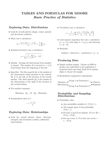
690TABLESTable entry for z is the area underthe standard Normal curve to theleft of z.Table entryzTABLE AStandard Normal cumulative proportionsz.00.01.02.03.04.05.06.07.08.09 3.4 3.3 3.2 3.1 3.0 2.9 2.8 2.7 2.6 2.5 2.4 2.3 2.2 2.1 2.0 1.9 1.8 1.7 1.6 1.5 1.4 1.3 1.2 1.1 1.0 0.9 0.8 0.7 0.6 0.5 0.4 0.3 0.2 0.1 641
TABLES691Table entryTable entry for z is the area underthe standard Normal curve to theleft of z.zTABLE AStandard Normal cumulative proportions (continued 74.9981.9986.9990.9993.9995.9997.9998
692TABLE BTABLESRandom 8869203316
Table entry for C is the criticalvalue t required for confidencelevel C. To approximate one- andtwo-sided P -values, compare thevalue of the t statistic with thecritical values of t that matchthe P -values given at the bottomof the table.TABLE CArea C t*Tail area 1 C2t*t distribution critical valuesCONFIDENCE LEVEL CDEGREES 30405060801001000z 3.4163.3903.3003.291One-sided ded P.50.40.30.20.10.05.04.02.01.005.002.001693
694TABLESTable entry for p is the criticalvalue χ with probability p lyingto its right.Probability pχ*TABLE DChi-square distribution critical 76.0989.56102.7128.3153.2
TABLESTable entry for p is the criticalvalue r of the correlation coefficient r with probability p lyingto its right.695Probability pr*TABLE ECritical values of the correlation rUPPER TAIL PROBABILITY 00.57030.50070.45140.41430.36110.32420.1039
Two-sided p-values for t-distributionabsolutevalue t .0170.0150.0130.0120.0110.0100.0100.009d.f. (1-15)Prepared by Professor James Higgins, Kansas State University
Two-sided p-values for t-distributionabsolutevalue t f. (16-30)Prepared by Professor James Higgins, Kansas State University
Sampling distribution of a sample mean: x has mean µ and standard deviationσ/ n. x has a Normal distribution if the popula- tion distribution is Normal. Central limit theorem: x is approximately Normal when n is large. Basics of Inference z confidence interval for a population mean (σ known, SRS from Normal population):x z σ n z from N(0,1)