WIXLIB

Pattern ClassificationWing-Kin (Ken) MaDepartment of Electronic Engineering,The Chinese University Hong Kong, Hong KongELEG5481, Lecture 14Acknowledgment: Jiaxian Pan for helping prepare the slides.

Introduction Suppose that we are given 50 pictures1 of tigers, 50 pictures of dolphins, and 50picture of monkeys. From the given pictures, we learn how tigers, dolphins and monkeys look like. Now, given a new picture, we want to know whether it is tiger, dolphin, or amonkey.A tiger,a dolphin,or a monkey?1All photographs are taken from the Internet.1

Pattern classification problem setup Let X be set of all possible inputs and Y be the set of all classes. We are given a set of training examples (or training data) x1, x2, . . . , xm X . Each data point xi has been labeled to belong a certain class.y1, y2, . . . , ym Y be the class labels corresponding to x1, x2, . . . , xm.Let– For example, consider Y { 1, 1}. The data point xi belongs to class“ 1” if yi 1, and class “ 1” if yi 1. Let f : X Y be a classifier or decision function, which should do the following:– f (xi) yi for i 1, . . . , m, or, if not possible, maximizes the number oftraining examples satisfying f (xi) yi .– for a new data x X , predict its class by f (x). Goal: learn a good classifier from the training data {(xi, yi)}mi 1.2

Binary Classification by the Support Vector Machine (SVM) Consider the binary classification case. Let Y { 1, 1}. Consider a simple decision functionf (x) sign(wT x b)where w Rn and b R. This classifier is known as the SVM. Problem 1: given {(xi, yi)}mi 1, find (w, b) such thatyi sign(wT xi b), i 1, . . . , m.( ) Eq. ( ) is equivalent towT xi b 0, if yi 1,wT xi b 0, if yi 1,for i 1, . . . , m. Or, we can writeyi(wT xi b) 0,i 1, . . . , m.3

Problem 1 can be written asfind w, bs.t. yi(wT xi b) 0, i 1, . . . , m,which is an LP feasibility problem. Geometrically, the problem is to find a hyperplane H {x wT x b 0} thatseparates the data {xi yi 1} from {xi yi 1}.4

A Robust SVM Formulation Suppose that there are uncertainties in {xi}mi 1, say, due to noise and modelingerrors. Under such cases, the classifier design in Problem 1 is not robust. Consider the spherical uncertainty model:x̃i xi ei,keik2 ρ,for i 1, . . . , m, where xi now denotes the “nominal” data point; x̃i the “true”data point; ei the corresponding uncertainty vector; ρ the uncertainty level.5

We wish to maximize the uncertainty level while still separating the data. Problem 2:max ρw,b,ρs.t. yi(wT (xi ei) b) 0, for all keik2 ρ, i 1, . . . , m.6

A recap of problem 2:max ρw,b,ρs.t. yi(wT (xi ei) b) 0, for all keik2 ρ, i 1, . . . , m. By the Cauchy-Schwarz inequality, we haveinfkei k2 ρyi(wT (xi ei) b) 0 yi(wT xi b) ρkwk2 0. Problem 2 is homogeneous—if (w , b ) is a solution, then (α · w , α · b ), forany α 0, is also a solution. Assume w.l.o.g. that ρkwk2 1. Problem 2 can be reformulated asmin kwk22w,bs.t. yi(wT xi b) 1, i 1, . . . , m.7

Alternative (and classical) Interpretation Define hyperplanes H {x wT x b 1} and H {x wT x b 1}. The distance between H and H is 2/kwk2. Problem 2 is identical to that of maximizing the distance between the parallelhyperplanes H and H .8

The Non-Separable Data Case A given training data set {(xi , yi)}mi 1 is not always separable; i.e., there doesnot exist a hyperplane that separates {xi yi 1} and {xi yi 1}. As a compromise, a minimum “loss” should be sought.9

A Soft Margin SVM Formulation Let ψ : R {0, 1} be a step loss function:ψ(x) 0, x 01, x 0. Problem 3 (an ℓ0-norm-like soft margin SVM):min kwk22 λ ·w,bmXψ(1 yi(wT xi b))i 1for some constant λ 0.– we design an SVM whose number of class-violated data points is small.– the problem is also robust against mislabeled data points.– the problem has a sparse opt. flavor. Problem 3 is nonconvex, owing to ψ (the same problem as in ℓ0 norm).10

Like sparse opt., a compromise is to approximate ψ by a more manageablefunction. As an example, consider the hinge loss function: 0, x 0h(x) x, x 0.h is convex. Also, note that h(x) max{0, x}. ℓ1-norm-like soft margin SVM:min kwk22 λ ·w,bmXmax{0, 1 yi (wT xi b)}.i 1The problem above can be reformulated as an SOCP (or convex QP):min kwk22 λ ·w,b,ξmXmax{0, ξi}i 1s.t. ξi 0, ξi 1 yi(wT xi b), i 1, . . . , m.Note: the above problem is the classical SVM formulation.11

Variations of SVM Formulations One may consider other approximate functions for ψ (e.g., the logistic regressionTloss log(1 e yi(w xi b)) ). One may also modify the uncertainty model.– For example, consider an interval uncertainty keik ρ.– The resulting SVM problem (with ℓ1-norm-like soft margin):min kwk1 λ ·w,bmXmax{0, 1 yi(wT xi b)}.i 1– Alternative interpretation: Since kwk1 approximates kwk0, the above SVMproblem has a flavor of choosing the smallest of elements (or features) toperform classification.12

Nonlinear SVM SVM restricts itself to the use of linear decision regions.– pros: “easy” to optimize.– cons: there are many cases where linear decision regions are not adequate. A possible remedy is to introduce a nonlinear mapping φ(x) to map data into adifferent space, and then construct a linear classifier in that space.13

Nonlinear SVM problemmin kwk22 λ ·w,b,ξmXξii 1s.t. yi(wT φ(xi) b) 1 ξi, ξi 0, i 1, . . . , m.where φ : Rn Rl is a predefined nonlinear mapping. This problem is still an SOCP, though a nonlinear mapping is applied to data xi. In practice, the dimension l of φ(x) can be very large or even infinite. This cancause significant problems in storing data in memory and solving the SOCP.14

The Representer Theorem The representer theorem [Shawe-Taylor and N. Cristianini’04] states that thereis an optimal solution w of the nonlinear SVM problem such thatw mXαiφ(xi)i 1for some α Rm. The representer thm. suggests that w Rl lies in some low dimensional spacespanned by {φ(xi)}mi 1, though the dimension l could be huge or even infinite. The nonlinear SVM problem is transformed tominw,b,α,ξkwk22 λ·Pmi 1 ξis.t. yi (wT φ(xi) b) 1 ξi , ξi 0, i 1, . . . , m,Pmw i 1 αiφ(xi).15

The Kernel Trick By direct substitution w, the nonlinear SVM problem can further be rewritten asTmin α Qα λ ·b,α,ξs.t. yi(PmPmj 1αj Qiji 1 ξi b) 1 ξi, ξi 0, i 1, . . . , m,Twhere Q SmwithQ φ(x)φ(xj ).iji To obtain Q, we do not need φ(xi) explicitly. We only need the inner productsφ(xi)T φ(xj ). There is no need to explicitly define the transform φ(x). Instead, we specify theso-called kernel function K(x, x′) φ(x)T φ(x′). Popular choice of kernel:K(x, x′) exp( δkx x′k2)K(x, x′) (xT x′/a b)d(Radial basis function)(Polynomial kernel)16

The Decision Function under the Kernel Trick The decision function is written as T f (x) sign (w ) x bPm sign ( i 1αi K(x, xi) b ) . The decision function is again specified by the kernel function K(x, x′) only.17

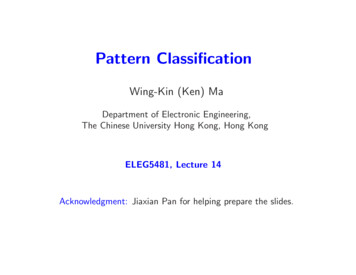
A toy example Six data points: ( 3, 3), (0, 1), (1, 1) are of class 1,and ( 1.5, 1.5), (2, 2), (0, 3) are of class 1. Nonlinear SVM with regularization λ 0.5. Radical basis function with δ 0.2. The black line is the decision boundary.43210 1 2 3 4 4 3 2 10123418

Maximum-Ratio Separating Ellipsoids (MRSEs) SVM employs linear decision regions. One can also consider ellipsoidal decision regions.19

Consider a K-class classification problem with Y {1, . . . , K}. Define the ellipsoidal set as E(u, P ) {x (x u)T P (x u) 1}, where u isthe center and P 0. For each class k Y, the objective is to find an ellipsoid E(uk , Pk ) and a scaledellipsoid E(uk , Pk /ρk ) with ρk 1 such that(xi E(uk , Pk ),if yi k,xi / E(uk , Pk /ρk ), if yi 6 k.20

The scaling factor ρk should be maximized, as ρk can be considered as themargin between class k and all other classes. The MRSE optimization problem:max ρk λ1 log det PkPk ,uk ,ρks.t. (xi uk )T Pk (xi uk ) 1,if yi k,(xi uk )T Pk (xi uk ) ρk , if yi 6 k,ρk 1,Pk 0,for k 1, . . . , K, where a regularization λ1 log det Pk with λ1 0 is added tothe objective function to ensure that the ellipsoid is non-degenerate, i.e., Pk 0. If the optimal ρk satisfies ρk 1, then the training data of class k can beperfectly separated from those of other classes.21

The MRSE problem is not convex, but can be transformed to a convex problemby a technique called homogeneous embedding.max ρk λ1 log det Φ11Φk ,ρks.t. ziT Φk zi 1,if yi k,ziT Φk zi ρk , if yi 6 k, Φφ12Φk T11 0,φ12 φ22Φk 0,where zi [xTi , 1]T . Pk and u k can be recovered byPk Φ 11/(1 δ ),u k (Φ 11) 1 φ 12, δ φ 22 (φ 12)T (Φ 11) 1φ 12.22

For the case of non-separate data, the same soft margin formulation in SVMcan be used:Pmax ρk λ1 log det Φ11 λ2 iξiΦk ,ρk ,ξs.t. ziT Φk zi 1 ξi,if yi k,ziT Φk zi ρk ξi, if yi 6 k, Φφ12Φk T11,φ12 φ22Φk 0,γi 0, for all i,where λ2 0 is some positive regularization parameter.23

Classification Rule Suppose in the training phase, we have solved the MRSE problem for eachk {1, . . . , K}. Given a new data x, define the score of class k as(x u k )T Pk (x u k )p sk .ρk The score sk measures how closed x is to class k. Choose the class that has the minimum score:k̂ argmink 1,.,Ksk .24

ReferenceA. Ben-Tal, L. El-Ghaoui, and A. Nemirovski, “Robust Optimization”, PrincetonUniversity Press, 2009.L. Xiao and L. Deng, “A geometric perspective of large-margin training of GaussianModels”, IEEE Trans. Signal Process. Mag., 2010.J. Shawe-Taylor and N. Cristianini, “Kernel Methods for Pattern Analysis”,Cambridge University Press, Cambridge, 2004.K. Q. Weinberger, F. Sha, and L. K. Saul, “Convex optimization for distance metriclearning and pattern classification,” IEEE Signal Process. Mag., May. 2010.25

Pattern Classification Wing-Kin (Ken) Ma Department of Electronic Engineering, The Chinese University Hong Kong, Hong Kong ELEG5481, Lecture 14 Acknowledgment: Jiaxian Pan for helping prepare the slides. Introduction Suppose that we are given 50 pictures1 of tigers, 50 pictures of dolphins, and 50