Transcription
Solutions to “Pattern Classification” by Duda et al.tommyod @ githubDecember 11, 2018AbstractThis document contains solutions to selected exercises from the book “PatternRecognition” by Richard O. Duda, Peter E. Hart and David G. Stork. Although itwas written in 2001, the second edition has truly stood the test of time—it’s a muchcited, well-written introductory text to the exciting field of pattern recognition(orsimply machine learning). At the time of writing, the book has close to 40 000citations according to Google.While short chapter summaries are included in this document, they are not intended to substitute the book in any way. The summaries will largely be meaninglesswithout the book, which I recommend buying if you’re interested in the subject.The solutions and notes were typeset in LATEX to facilitate my own learningprocess. Machine learning has rightfully garnered considerable attention in recentyears, and while many online resources are worthwhile it seems reasonable to favorbooks when attempting to learn the material thoroughly.I hope you find my solutions helpful if you are stuck. Remember to make anattempt at solving the problems yourself before peeking. More likely than not,the solutions can be improved by a reader such as yourself. If you would like tocontribute, please submit a pull request at https://github.com/tommyod/lml/.Figure 1: The front cover of [Duda et al., 2000].1
Contents1 Notes from “Pattern Classification”1.2 Bayesian Decision Theory . . . . . . . . . . . . . . . . .1.3 Maximum-likelihood and Bayesian parameter estimation1.4 Nonparametric techniques . . . . . . . . . . . . . . . . .1.5 Linear discriminant functions . . . . . . . . . . . . . . .1.6 Multilayer Neural Networks . . . . . . . . . . . . . . . .1.7 Stochastic methods . . . . . . . . . . . . . . . . . . . . .1.8 Nonmetric methods . . . . . . . . . . . . . . . . . . . . .1.9 Algorithm-independent machine learning . . . . . . . . .1.10 Unsupervised learning and clustering . . . . . . . . . . .2 Solutions to “Pattern Classification”2.2 Bayesian Decision Theory . . . . . . . . . . . . . . . . .2.3 Maximum-likelihood and Bayesian parameter estimation2.4 Nonparametrix techniques . . . . . . . . . . . . . . . . .2.5 Linear discriminant functions . . . . . . . . . . . . . . .2.6 Multilayer Neural Networks . . . . . . . . . . . . . . . .2.7 Stochastic methods . . . . . . . . . . . . . . . . . . . . .2.8 Nonmetric methods . . . . . . . . . . . . . . . . . . . . .2.9 Algorithm-independent machine learning . . . . . . . . .2.10 Unsupervised learning and clustering . . . . . . . . . . .2.333567891112.14142334404855586469
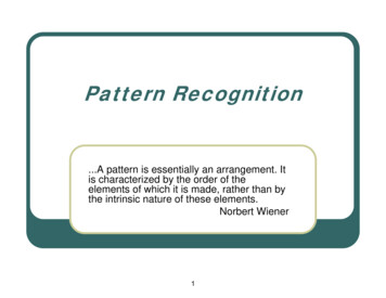
1Notes from “Pattern Classification”1.2Bayesian Decision Theory Bayes theorem isP (ωj x) likelihood priorp(x ωj ) P (ωj ) .p(x)evidenceThe Bayes decision rule is to choose the state of nature ωm such thatωm arg max P (ωj x).j Loss functions (or risk functions) with losses other than zero-one are possible. Ingeneral, we choose the action λ to minimize the risk R(λ x). The multivariate normal density (the Gaussian) is given by 11T 1exp (x µ) Σ (x µ) .p(x µ, Σ) 2(2π)d/2 Σ 1/2It is often analytically tractable, and closed form discriminant functions exist. If features y are missing, we integrate them out (marginalize) using the sum ruleZZp(x) p(x, y) dy p(x y)p(y) dy. In Bayesian belief networks, influences are represented by a directed network. If Bis dependent on A, we add a directed edge A B to the network.Figure 2: A Bayesian belief network. The source is Wikipedia.1.3Maximum-likelihood and Bayesian parameter estimation The maximum likelihood of a distribution p(x θ) is given by θ̂ arg maxθ p(D θ),assuming i.i.d. data points and maximizing the log-likelihood, we haveθ̂ arg max ln p(D θ) arg max lnθθnYp(xi θ).i 1Analytical solutions exist for the Gaussian. In Rgeneral a maximum likelihood estimate may be biased, in the sense that Ex [θ̂] θ̂p(x) dx 6 θ.3
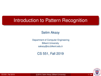
In the Bayesian framework, the parameter θ is expressed by a probability densityfunction p(θ). This is called the prior distribution of θ, which is updated when newdata is observed. The result is called the posterior distribution, given byp(θ D) p(D θ)p(θ)p(D θ)p(θ) R.p(D)p(D θ)p(θ) dθThe estimate of x then becomesZZZp(x D) p(x, θ D) dθ p(x θ, D)p(θ D) dθ p(x θ)p(θ D) dθ, which may be interpreted as a weighted average of models p(x θ), where p(θ D)is the weight associated with the model.The Bayesian framework is analytically tractable when using Gaussians. For instance, we can compute p(µ D) if we assume p(µ) N (µ0 , Σ0 ). The distributionp(µ) is called a conjugate prior and p(µ D) is a reproducing density, since a normalprior transforms to a normal posterior (with different parameters) when new datais observed.In summary the Bayesian framework allows us to incorporate prior information,but the maximum-likelihood approach is simpler. Maximum likelihood gives us anestimate θ̂, but the Bayesian framework gives us p(θ D)—the full distribution.Principal Component Analysis (PCA) yields components useful for representation.The covariance matrix is diagonalized, and low-variance directions in the hyperellipsoid are eliminated. The computation is often performed using the Singular ValueDecomposition (SVD).Discriminant Analysis (DA) projects to a lower dimensional subspace with optimaldiscrimination (and not representation).Expectation Maximization (EM) is an iterative algorithm for finding the maximumlikelihood when data is missing (or latent).Figure 3: A hidden Markov model. The source is Wikipedia. A discrete, first order, hidden Markov model consists of a transition matrix A and anemission matrix B. The probability of transition from state i to state j is given by4
aij , and the probability that state i emits signal j is given by bij . Three fundamentalproblems related to Markov models are:– The evaluation problem - probability that V T was emitted, given A and B.– The decoding problem - determine most likely sequence of hidden states ω T ,given emitted V T , A and B.– The learning problem - determine A and B given training observations of V Tand a coarse model.1.4Nonparametric techniques Two conceptually different approaches to nonparametric pattern recognition are:– Estimation of densities p(x wj ), called the generative approach.– Estimation of P (wj x), called the discriminative approach. Parzen-windows (kernel density estimation) is a generative method. It places akernel function φ : R R on every data point xi to create a density estimate nkx xi kp1X 1φ,pn (x) n i 1 Vnhnwhere k·kp : Rd R is the p-norm (which induces the so-called Minkowski metric)and hn 0 is the bandwidth. k-nearest neighbors is a discriminative method. It uses information about the knearest neighbors of a point x to compute P (wj x). This automatically uses moreof the surrounding space when data is sparse, and less of the surrounding spacewhen data is dense. The k-nearest neighbor estimate is given by# samples labeled wj.P (wj x) k The nearest neighbor method uses k 1. It can be shown that the error rate P ofthe nearest neighbor method is never more than twice the Bayes error rate P incthe limit of infinite data. More precisely, we have P P P (2 c 1P ). In some applications, careful thought must be put into metrics. Examples includeperiodic data on R/Z and image data where the metric should be invariant to smallshifts and rotations. One method to alleviate the problems of using the 2-norm as ametric on images is to introduce the tangent distance. For an image x0 , the tangentvector of a transformation F (such as rotation by an angle αi ) is given byT Vi F (x0 ; αi ) x0 .If several transformations are available, their linear combination may be computed.For each test point x, we search the tangent space for the linear combination minimizing the metric. This gives a metric D(x, x0 ) which is invariant to transformationssuch as small rotations and translations, compared to the 2-norm. Reduced Coloumb energy networks use ideas from both Parzen windows and knearest neighbors. It adjusts the size of the window so that it is less than somemaximal radius, while not touching any observation of a different class. This creates “basins of attraction” for classification.5
1.5Linear discriminant functions A linear discriminant function splits the feature space in two using a hyperplane.The equation for a hyperplane is given by 1TTg(x) ω x ω0 a y ω0 ω,xwhere ω0 is the bias. The expression aT y is called the augmented form.Figure 4: Linear discriminant functions. The source is Wikipedia. A linear machine assigns a point x to state of nature ωi ifgi (x) gj (x)for every other class j. This leaves no ambiguous regions in the feature space. By introducing mappings y h(x) to higher- or lower-dimensional spaces, nonlinearities in the original x-space may be captured by linear classifiers working iny-space. An example is y h(x) exp( xT x) if data from one class is centeredaround the origin. Another example is transforming periodic data with period Pfrom 0 x P to y by use of the functionsy1 cos (2πx/P )y2 sin (2πx/P ) . Several algorithms may be used to minimize an error function J(a). Two popularchoices are gradient descent and Newton descent.– Gradient descent moves in the direction of the negative gradient. It is oftencontrolled by a step length parameter η(k), which may decrease as the iterationcounter k increases. The update rule is given bya a η(k) J(a).– Newton descent also moves in the direction of the negative gradient, but theoptimal step length is computed by linearizing the function J(a) (or, equivalently, a second order approximation of J(a)). The update rule is given bya a H 1 J(a).6
Criterion functions for linearly separable data sets include:P– The Perceptron function y Y ( aT y), which is not smooth.P– The squared error with margin, given by y Y (aT y b)2 / kyk2 . The Mean Squared Error (MSE) approach may be used, but it is not guaranteed toyield a separating hyperplane—even if one exists. 1 T– The MSE solution is found analytically by the pseudoinverse A† AT AA .The pseudoinverse should never be used explicitly because it’s numericallywasteful and unstable. It represents the analytical solution to the problemmin eT e min (b Ax)T (b Ax) ,xxwhich is solved by x A† b.– The MSE approach is related to Fisher’s linear discriminant for an appropriatechoice of margin vector b.– LMS may be computed using matrix procedures (never use the pseudoinversedirectly) or by the gradient descent algorithm.– Ho-Kashyap procedures will return a separating hyperplane if one exists. Linear programming (LP) may also be used to find a separating hyperplane. Severalreductions are possible by introducing artificial variables.– Minimizing the Perceptron criterion function may be formulated as an LP, andthe result is typically decent even if a separating hyperplane does not exist. Support Vector Machines (SVM) find the minimum margin hyperplane. This is aquadratic programming (QP) problem, and the dual problem is easier to solve thanthe primal problem.1.6Multilayer Neural NetworksFigure 5: A three-layer neural network with bias. The source is Wikipedia. The feedforward operation on a d nH c three-layer neural network is defined bythe following equation for the output!!nHdXXzk fwkj fwji xi wj0 wk0 .j 1i 17
1.7- The Kolmogorov-Arnold representation theorem implies that any continuous function from input to output may be expressed by a three layer d nH c neuralnetwork with sufficiently many hidden units.Backpropagation learns the weights w by the gradient descent equation wn 1 wn η J(wn ). The gradient, or derivative, is found by repeated application of thechain rule of calculus. Several protocols are available for backpropagation: stochastic, batch and on-line.– Backpropagation may be thought of as feature mapping. While the inputs xiare not necessarily linearly separable, the outputs yj of the hidden units becomelinearly separable as the weights are learned. The final linear discriminantworks on this data instead of the xi .Practical tips for improving learning in neural networks include: standardizing features, adding noiseinitializing weights to random values and data augmentations,in the range 1/ d wji 1/ d, using momentum in the gradient descent algorithm, adding weight decay (equivalent to regularization) while learning, trainingwith hints (output units which are subsequently removed) and experimenting withvarious error functions.Second order methods for learning the weights include– Newtons method – uses H in addition to J(w).– Quickprop – two evaluations of J(w) to approximate a quadratic.– Conjugate gradient descent – uses conjugate directions, which consists ofa series of line searches. A given search direction does not spoil the result ofthe previous line searches. This is equivalent to a “smart momentum.”Other networks include:– Convolutional Neural Networks (CNNs) – translation invariant, has achievedgreat success on image data.– Recurrent Neural Networks (RNNs) – the output of the previous prediction isfed into the subsequent prediction. This simulates memory, and RNNs havebeen successful on time series data.– Cascade correlation – a technique where the topology is altered by adding moreunits until the performance is sufficiently good.Stochastic methods Stochastic methods are used to search for optimal solutions when techniques suchas gradient descent are not viable. For instance if the model is very complex, has adiscrete nature where gradients are not available, or if there are time constraints. Simulated annealing is an optimization technique. As an example: to minimize theerror E(s), where s [ 1, 1]n , we change a random entry of s.– If the change produces a better result, then keep the new s.– If the change does not produce a better result, we still might keep the change.The probability of keeping a change which increases the error E(s) is a functionof the temperature T , which typically decreases exponentially as the algorithm pro8
gresses. Initially simulated annealing is a random search, and as the temperatureprogresses it becomes a greedy search. Deterministic simulated annealing replaces discrete si with analog (continuous) si .This forces the other magnets sk (k 6 i) to determine si i.si f (T, i ) tanhTAs T 0, the tanh(·) sigmoid function converges to a step function. Boltzmann networks (or Boltzmann machines) employ simulated annealing in a network to make predictions. First, weights wij are learned so that inputs sj αilead to correct outputs sk αo during classification. In the classification phase, theinputs αi are clamped (fixed), and simulated annealing produces outputs αo . If theweights wij are learned correctly, then the algorithm will produce good classifications.– Boltzmann networks are able to perform pattern completion.Figure 6: A non-restricted Boltzmann machine. The source is Wikipedia. Evolutionary methods take a population of classifiers through many generations. Ineach generation, new classifiers (offspring) are produced from the previous generation. The best classifiers are subject to (1) replication, (2) crossover and (3) mutation to produce offspring. The classifiers may be encoded as 2-bit chromosomes oflength L. The bits represent some property of the classifier. Genetic programming is the process of modifying formulas such as[( x1 ) x2 ] / [(ln x3 ) x2 ]by evolutionary methods, mutating variables and operators and performing crossovers.1.8Nonmetric methods A decision tree typically splits the feature space along the axes if the data is numeric,and works well for non-metric (categorical, or nominal) data as well. To implementa decision tree, one must consider– The number of splits made per node (typically 2, since a higher branchingfactor B may be reduced to B 2 anyway).9
– How to choose an attribute to split on – often solved using information gain.– When a node should be declared a leaf node.– How to handle missing data. To decide which attribute to split on, an impurity function is defined for a nodeN consisting of training samples from various categories ω1 , . . . , ωC . The impurityfunction should be 0 when all samples in node N are from the same category ωj ,and peak when the samples are uniformly drawn from the C categories.Two examples of impurity functions are entropy impurity and Gini impurity, whichare respectively defined asi(N ) CXP (ωj ) ln P (ωj )i(N ) j 1CXj 1P (ωj )XP (ωk ) k6 jCXP (ωj ) [1 P (ωj )] .j 1A split is chosen so that it maximizes the decrease in impurity, i.e. i(N ) i(N ) [PL i(NL ) (1 PL ) i(NR )] .The above equation says that the change in impurity equals the original impurity atnode N minus the weighted average of the impurity of the left and right child node. Other considerations in decision trees include:– Pruning – simplifying the tree after training (bypassing the horizon effect).– Penalizing complexity – regularization of the tree structure.– Missing attributes – for instance using (1) surrogate splits or (2) sending atraining sample down every path and then performing a weighted average. Four string problems in pattern classification are:– Matching: naive matching is slow, the Boyer-Moore string matching algorithmis much more efficient. It operates by increasing the shift s of x using twoheuristics in parallel: the bad-character heuristic and the good-suffix heuristic.– Edit distance: a way to compare the “distance” between strings by countingthe number of insertions, deletions and substitutions required to transform xto y. If all costs are equal, then D(x, y) is a metric. A dynamic programingalgorithm is used to compute edit distance.– Matching with errors is the same as matching, but using for instance theedit distance to find approximate matches. The problem is to find a shift sthat minimizes the edit distance.– Matching with the “don’t care”-symbol : same as matching, but the -symbol matches any character in the alphabet A. A grammar G (A, I, S, P) consists of symbols A, variables I, a root symbol Sand productions P. Concrete examples include English sentences and pronunciationof numbers. There are several types of grammars, and they constitute a hierarchyType 3 Type 2 Type 1 Type 0.The types are respectively called regular, context free, context sensitive and free.– A central question is whether a string x is in the language L generated by thegrammar G, i.e. whether x L(G). This can be answered using bottom-upparsing, which employs the product rules P backwards.10
1.9Algorithm-independent machine learning The no free lunch theorem states that using the off-training set error, and assumingequally likely target functions F (x), no algorithm is universally superior. Anystatement about algorithms is a statement about the target function F (x). The ugly duckling theorem states that no feature representation is universally superior. If pattern similarity is based on the number of possible shared predicates (f1OR f2 , etc) then any two patterns are equally similar. The best feature representation consequently depends on the target function F (x). The minimum description length is a version of Occam’s razor. In this framework,the best hypothesis h (model) is the one compressing the data the most, i.e. theminimizer h ofK(h, D) K(h) K(D using h),where K(·) is the Kolmogorov complexity (length of smallest computer program). The bias-variance trade-off is exemplified by the equation ED (g(x; D) F (x))2 ED [g(x; D) F (x)]2 ED (g(x; D) E [g(x; D)])2 ,{z} {z}bias2varianceand informally states that there is always a trade-off between bias and variance. Inthe regression setting, the bias is the average error over many data sets, while thevariance is the variability of the estimate over many data sets. High variance typically implies many parameters (over-fitting), while high bias implies few parameters(under-fitting). The Jackknife re-sampling method involves removing the ith data point from D {x1 , x2 , . . . , xn } and computing a statistic. This is done for every data point, andthe final result is averaged. From this the variance of the statistic may be assessed. The bootstrap method involves re-samling n data points from Dn with replacementB times. The statistic is computed B times, and is then averaged.θ̂ (·) B1 X (b)θ̂B b 1varboot [θ̂] B 21 X (b)θ̂ θ̂ (·)B b 1 Bagging consists of taking an average over model predictions. Boosting uses theresult of model hn to train model hn 1 . Informally, the next model prioritizes datain D which the sequence of models so far has not performed well on.– Adaptive Boosting (AdaBoost) is a well known boosting algorithm. It samplesdata xi using probability weights wi . If a model hn does a poor job, theassociated weights win 1 are increased exponentially. This causes exponentialerror decay on training data. Learning with queries involves the model choosing the next data point to learn from.It assumes the existence of an oracle which can give the correct answer to any input,but using this oracle might be costly. Efficient learning involves choosing pointswhere the classifier is uncertain, i.e. where P (ω1 x) P (ω2 x).11
Maximum-likelihood model comparison picks the maximum of θP (D hi ) ' P (D θ̂, hi ) P (θ̂ hi ) θ P (D θ̂, hi ) 0 , {z} {z} θbest-fit likelihoodOccam factorwhere θ is the volume of the possible parameter space given the data D, and 0 θis the prior volume of the possible parameter before seeing data. Applying a fewsimplifications, this becomes a two step process: (1) compute maximum likelihoodestimate θ̂ from the data, then (2) compute the likelihood value given θ̂. Mixture models can be used to combineP classifiers using discriminant functions.The final discriminant function is g ki 1 wi gi (x, θi ), and an underlying mixturemodel of the following form is assumed:0p(y x, Θ ) kXr 11.10P (r x, θ00 ) p(y x, θr0 ){z} prob. of model rUnsupervised learning and clustering Unsupervised learning is a difficult problem. A mixture model may not be identifiable, which happens when θ cannot be determined uniquely even in the limit ofinfinite data. There exist necessary conditions for ML solutions to P̂ (ωi ) and θ̂i , butthey are not sufficient to guarantee that a maximum is found. Singular solutionsmay occur, since the likelihood can be made arbitrarily large when µi is placed ona data point and σi 0. A Bayesian approach is possible, but rarely feasible. The k-means algorithm is a simple procedure for finding µ1 , . . . , µk . A fuzzy kmeans algorithm also exists, in which membership categorization is not binary. It is better to find structure in data than to impose it. A metric d(·, ·) and adistance threshold d0 may be defined, which may then be used to group points.This approach is sensitive to the effect of individual data points. Standardizingdata using yi (xi µk )/σk may or may not be beneficial, and the same goes forPCA. Many criterion functions are available for clustering, e.g. sum of square errorJe c XXkx mi k2 .i 1 x DiCriterion functions based on the size of scatter matrices (LDA) are Je tr [SW ] ,Jd det [SW ] and Jf tr ST 1 SW . Hierarchical clustering represents hierarchical (clusters within clusters) structure ina dendrogram, see Figure 7 on page 13. Two approaches are possible: agglomerative(merging) og divisive (splitting). Many distance measures are available.– Using dmin (Di , Dj ) and agglomerative clustering, a minimal spanning tree (MST)is built from the data.12
Figure 7: A dendrogram representation of hierarchical clustering.Wikipedia.The source is Competitive learning is a clustering algorithm implemented by a neural network.The data x Rd is augmented to x : (1, x) and normalized so that it lies ona (d 1)-dimensional sphere. The weight w arg maxw wT x is updated to bemore similar to the sample x. The algorithm can also create new clusters wj ifcertain conditions are met. It’s suitable for on-line learning, but will not necessarilyconverge with constant learning rate. PCA can be implemented as a 3-layer neural network autoencoder. The first keigenvalues/eigenvectors of X solves the minimization of kX Xk0 k, where Xk0 isa rank k approximation of X. Non-linear PCA is an extension of the idea, using a5-layer non-linear neural network autoencoder.Figure 8: A neural network autoencoder with 5 layers. The source is Wikipedia. Self-organizing feature maps transform from a high dimensional space to low dimensional one, while preserving local topological information. They are implemented asneural networks, and a key idea is to update neighboring areas when learning themap. An additional benefit is that they automatically place more points in regionsof high probability.13
2Solutions to “Pattern Classification”This section contains solutions to problems in “Pattern Classification” by Duda et al.There are approximately 8 solved problems from each chapter.2.2Bayesian Decision TheoryProblem 2.6a) We want the probability of choosing action α2 to be smaller than, or equal to, E1 ,given that the true state of nature is ω1 . Let’s assume that µ1 µ2 and that thedecision threshold is x , so we decide α2 if x x . We then haveP (α2 ω1 ) E1p(x x ω1 ) E1 Z x 1 p(x ω1 ) dx E10We let Φ : R [0, 1] denote the cumulative Gaussian distribution, and Φ 1 :[0, 1] R it’s inverse function. Making use of Φ we write x µ11 Φ E1σ1x µ1 σ1 Φ 1 (1 E1 ) .If the desired error is close to zero, then x goes to positive infinity. If the desirederror is close to one, then x goes to negative infinity.b) The error rate for classifying ω2 as ω1 is Z x x µ2 P (α1 ω2 ) p(x x ω2 ) p(x ω2 ) dx Φ.σ20Making use of x from the previous problem, we obtain µ1 µ2 σ1 1µ1 σ1 Φ 1 (1 E1 ) µ2Φ Φ Φ (1 E1 ) .σ2σ2σ2c) The overall error rate becomesP (error) P (α1 , ω2 ) P (α2 , ω1 ) P (α1 ω2 )P (ω2 ) P (α2 ω1 )P (ω1 )1 [P (α1 ω2 ) P (α2 ω1 )]2 1µ1 µ2 σ1 1 E1 Φ Φ (1 E1 ) .2σ2σ214
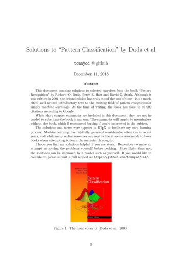
In the last equality we used the results from the previous subproblems.d) We substitute the given values into the equations, and obtain x 0.6449. Thetotal error rate is P (error) 0.2056.e) The Bayes error rate, as a function of x , is given byP (error) P (α2 ω1 )P (ω1 ) P (α1 ω2 )P (ω2 )1 [p(x x ω1 ) p(x x ω2 )] 2 1x µ1x µ2 1 Φ Φ2σ1σ2The Bayes error rate for this problem is depicted in Figure 9.0.50.4p(x 1)p(x 2)P(error)x*0.30.20.10.0432101234Figure 9: Graf accompanying problem 2.6.Problem 2.12a) A useful observation is that the maximal value P (ωmax x) is greater than, or equalto, the average. Therefore we obtainc1X1P (ωmax x) P (ωi x) ,c i 1cwhere the last equality is due to probabilities summing to unity.b) The minimum error rate is achieved by choosing ωmax , the most likely state of nature.The average probability of error over the data space is therefore the probability thatωmax is not the true state of nature for a given x, i.e.ZP (error) Ex [1 P (ωmax x)] 1 P (ωmax x)p(x) dx.c) We see that11c 1P (ωmax x)p(x) dx 1 p(x) dx 1 ,cccRwhere we have used the fact that p(x) dx 1.d) A situation where P (error) (c 1)/c arises when P (ωi ) 1/c for every i. Thenthe maximum value is equal to the average value, and the inequality in problem a)becomes an equality.ZZP (error) 1 15
Problem 2.19Ra) The entropy is given by H [p(x)] p(x) ln p(x) dx. The optimization problemgives the synthetic function (or Lagrange function) Z ZqXHs p(x) ln p(x) dx λkbk (x)p(x) dx ak ,k 1Rand since a probability density function has p(x) dx 1 we add an additionalconstraint for k 0 with b0 (x) 1 and ak 1. Collecting terms we obtainZZqqXXHs p(x) ln p(x) dx λk bk (x)p(x) dx λ k akZ k 0q"p(x) ln p(x) Xk 0#λk bk (x) dx k 0qXλk ak ,k 0which is what we were asked to show.b) Differentiating the equation above with respect to p(x) and equating it to zero weobtain"# !ZqX1 1 ln p(x) λk bk (x) p(x)dx 0.p(x)k 0This integral is zero if the integrand is zero for every x, so we require thatln p(x) qXλk bk (x) 1 0,k 0and solving this equation for p(x) gives the desired answer.Problem 2.21We are asked to compute the entropy of the (1) Gaussian distribution, (2) triangle distribution and (3) uniform distribution. Every probability density function (pdf) has µ 0and standard deviation σ, and we must write every pdf parameterized using σ.RGaussian We use the definition H [p(x)] p(x) ln p(x) dx to compute Z1 x211 x21H [p(x)] exp 2ln dx.2σ2 σ22πσ2πσ1Let us denote the constant by K 2πσto simplify notation. We obtain Z1 x21 x2 K exp 2ln K dx 2σ2 σ2 ZZ1 x21 x21 x2 K ln K exp 2 dx Kexp 2 dx2σ2 σ22σ16
The first term evaluates to ln K, since it’s the normal distribution with an additionalfactor ln K. The second term is not as straightforward. We change variables to y x/ 2σ , and write it asZ K y 2 exp y 2 2σ dy,and this integral is solved by using the following observation (from integration by parts):ZZ2 x2 x2 x( 2x)e x dx.1edx xe {z }0 at Using the above equation in reverse, we integrate as follows: 1Z Z 2 1 12K 2σ y exp y dy K 2σπ exp y 2 dy K 2σ222To recap, the first integral evaluated to ln K, and the second evaluated to entropy of the Gaussian is therefore 1/2 ln 2πσ.1.2TheTriangle The triangle distribution may be writt
Solutions to \Pattern Classi cation" by Duda et al. tommyod @ github December 11, 2018 Abstract This document contains solutions to selected exercises from the book \Pattern Recognition" by Richard O. Duda, Peter E. Hart and David G. Stork. Although it was written in 2001, the sec