WIXLIB

Coupled PDEs with Initial Solution from Data in COMSOL 4X. Huang, S. Khuvis, S. Askarian, M. K. Gobbert , and B. E. PeercyDepartment of Mathematics and Statistics, University of Maryland, Baltimore County Corresponding author: 1000 Hilltop Circle, Baltimore, MD 21250, gobbert@umbc.edua cell given by the square domain Ω (0, 150) (0, 150) R2 in units of micrometers (µm) isdescribed mathematically by this reduced systemof coupled time-dependent reaction-diffusion equations for all (x, y) Ω with no-flow boundaryconditions n · (Deff C) 0 for all (x, y) Ω.The initial conditions are given by data in txtfiles that specify the values of C(x, y, 0) C0 (x, y)and v(x, y, 0) v0 (x, y) on a 50 50 mesh of Ω.The physiological parameters of the problem areDeff 1, α β 0.1, γ 0.2, and 0.07.The first PDE for the excitation variable is atime-dependent reaction-diffusion equation representing the excitable dynamic, and the secondPDE for the recovery variable controls the local recovery of the excitation. The second PDE does nothave any diffusivity term, and the C-dependence isthe only reason for spatial dependence of the recovery variable. The zero-flux boundary condition isapplied for the first PDE. We choose a final timeof tfin 350 seconds.Abstract: Many physical applications requirethe solution of a system of coupled partial differential equations (PDEs). In most cases the analytic PDE solution does not exist for this systemand we need to solve the problem numerically using the finite element method in COMSOL. Thispaper presents information on techniques neededin COMSOL 4 to enable computational studies ofcoupled systems of PDEs for time-dependent nonlinear problems. Furthermore, we demonstratehow to use data files as input for initial conditions. To illustrate the techniques, we considera system of two time-dependent non-linear PDEsfrom mathematical biology.Keywords: System of PDEs, Coupled PDEs,Reaction-diffusion equation, Initial condition.1IntroductionThis paper extends the step-by-step instructionsin [3, 4] for solving one stationary linear PDE toa system of time-dependent non-linear PDEs. Wepresent two different approaches in COMSOL tosolve coupled systems of PDEs. In the first approach, each equation in the coupled system ofPDEs is modeled independently in its own Physicsmodel, and then they are coupled together. In thesecond approach, the matrix form of coefficients isused to specify all PDEs of the coupled system inone Physics model. This approach is appropriateif all PDEs have the same form. Furthermore, thetechnique to read initial solution from a data fileinto COMSOL 4 is introduced.To illustrate how to set up coupled PDEs withinitial solution from a data file, we present an example from mathematical biology, the FitzHughNagumo equations [1]2Use of COMSOL 4 to SolveCoupled System of PDEIn this section, we illustrate the instruction of solving a coupled system of PDE in COMSOL 4. Twoapproaches are used to solve the coupled systemand we provide instructions for both of these approaches in Sections 2.1 and 2.2. This is followedin Section 2.3, where the methods of reading datain txt files and using them as initial conditions areintroduced. As the last step, the post-processingof solutions including changing the appearance ofplots is presented in Section 2.4.2.1Ct · (Deff C) C(C α)(1 C) βv,Approach One: Each PDE in itsown Physics ModelIn this section, the step by step instructions to(1) solve the coupled diffusion problem using the firstapproach are given. The idea of the first approachinspired by a recent study of calcium dynamics [2]. is to model each PDE equation in the system sepThe spread of excitation variable C(x, y, t) through arately and then couple them together.vt (C γv),1

default zero flux boundary condition is used andthe initial condition is in the form of 2 1 vectorwith C0 (x, y) and v0 (x, y) as the elements.To start the model, look for Model Wizard in themiddle panel, choose 2D, Coefficient Form PDE,Time Dependent, and then click the Finish flag.To solve any system of equations it is required tocreate Geometry of domain. In our case, we createa square domain of the size 150 150. In the nextstep, the appropriate Physics should be added tothe Model tab. Each equation in the coupled system of PDEs is represented by one Physics addedto the model. We now already have one physics asCoefficient Form PDE, we can use it for the firstequation in (1). Here the unknown is C(x, y, t),representing the excitation variable. The righthand side C(C α)(1 C) βv is specified as sourceterm. Notice that the other variable v is coubledhere. Next we need to specify the boundary condition, in this case the default zero flux boundarycondition is used. Initial Condition C0 (x, y) is notconstant and its value has been provided as datafile. Reading initial condition to Initial Valuesof the PDE is not straightforward and is explainedin the next section.Now, to add our second equation, right clickModel 1 and select Add Physics, choose alsoCoefficient Form PDE, Time Dependent, andthen click the Finish flag.We can selectthis second Coefficient Form PDE (c2) tab, andchange the name of dependent variables to v, representing the recovery variable. It is straightforwardto specify the source term (C γv) and the initialcondition just like for the first equation.Finally, the mesh has been set up asPhysics-Controlled mesh, and computation isperformed to tfin 350.2.3Setting up Initial Conditionsfrom Data FilesThe initial condition profiles for the excitationvariable, C0 (x, y), and recovery variable, v0 (x, y),are provided in two separate txt files. A singleline of each of these files has three columns, containing the coordinate x, the coordinate y, and theinitial value at (x, y). In order to use these initialconditions in the system of PDEs, we create afunction for each of the variables. To create thesefunctions, right click on Global Definitionsand select Interpolation Function.Inthe Interpolation Function window forData source select File and import the appropriate txt file. The data format should bespreadsheet if the file is of the form describedabove, otherwise a different file format will benecessary. The number of arguments for thismodel is 2, since we have the x and y coordinatesfor each value. The position in file is 1 sincethere is only one species value in this file. Finally,Use space coordinates as arguments field isselected with Mesh as Frame.In this way, two interpolation functions are created, one for each of the variables. In order to usethese intial values in the system of PDEs, enterthe name of the appropriate interpolation functionas the initial value for the dependent variable inInitial Values 1. The initial condition profilesof excitation variable C and recovery variable v are2.2 Approach Two: Coupled PDEs illustrated in Figures 2 (a) and 3 (a), respectively.Figure 1 is a plot of our mesh, notice that the iniin one Physics Modeltial condition does not have to agree to the meshIn the second approach, the idea is to use only grid, since we are using interpolation.one Physics and represent the coupled system ofPDEs by using the matrix forms of coefficients. In 2.4 Post-Processingthis example, Physics, Coefficient Form PDE isadded to the model and two dependent variables C The two approaches above generated identical reand v are defined, it is crucial that the coefficients sults, allowing us to believe the same model is beare set such that they represent ((1)) correctly. In ing built. In this section, we show how to viewthis case, Diffusion Coefficient is a diagonal and output results. After the computation is done,2 2 matrix with 1 and 0 on diagonal. The source right click on Results and add 2D Plot Group. Interm is a 2 1 vector with f1 C(C α)(1 2D Plot Group, we select solution set, and timeC) βv and f2 (C γv) as sources for first that we would like to plot the result. Right clickand second PDE, respectively. For this example on 2D Plot Group node and add Surface, in dataall other coefficient matrices are sparse. Again the set we choose the same solution set and use C or v2

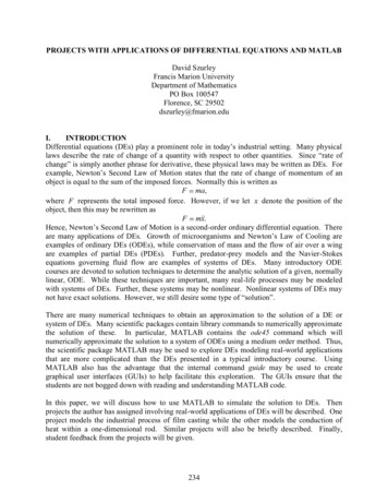
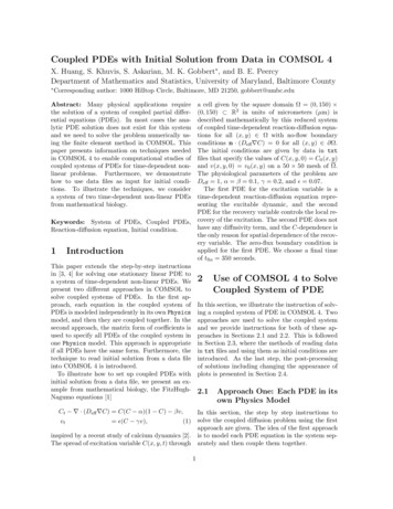
pattern. This physiological process is characterized by the visual appearance of a double ‘spiralwave’, a reaction-diffusion wave of the excitationvariable that moves through the domain in a spiraling, recurrent way. The close resemblance ofresults at times t 0 and t 300 seconds as wellas t 50 and t 350 seconds, in particular visible in Figure 4, bear out that the process has anapproximate period of 300 seconds. This explainsour choice of the final time of tfin 350 seconds.AcknowledgmentsFigure 1: Mesh of the square domain.The hardware used in the computational studies is part of the UMBC High Performance Computing Facility (HPCF). The facility is supportedby the U.S. National Science Foundation throughthe MRI program (grant nos. CNS–0821258 andCNS–1228778) and the SCREMS program (grantno. DMS–0821311), with additional substantialsupport from the University of Maryland, Baltimore County (UMBC). See www.umbc.edu/hpcffor more information on HPCF and the projectsusing its resources. Co-author Huang also acknowledges financial support as HPCF RA.as the expression to plot. We can manually set therange by clicking manual color range. To createa 3d view of the surface, we right click on Surfacenode and add Height Expression. In order to setthe scale to real value, we use 0.01 scale factor withzero offset. We can repeat this procedure for eachtime step.3ResultsWe have demonstrated two different approaches inSection 2 to solve the coupled system of PDEs in(1), and discussed how to setup initial conditionsusing txt files. For smaller systems of coupledPDE (with two or three dependent variables), thefirst approach is convenient to apply. However, forlarger systems which have more dependent variables of the same type, it is suggested to use thematrix form of coefficients to represent the wholesystem in one Physics, Coefficient Form PDE.Figures 2 and 3 depict the three-dimensionalview of the excitation variable and recovery variable, respectively, at time steps 0, 50, 100, . . . ,350 seconds. In the initial frame, excitation is induced (interior peak), and simultaneously the corner of the domain is excited analogous to a burnline to thwart a forest fire in a given direction. Consequently, propagation of the excitation proceedsinto the resting part of the domain. A recoveryvariable controls the local recovery of the excitation. The recovery is slow, but rapid enough for thecorners of the domain adjacent to the burn line tobegin to curl into the newly recovered region. Figure 4 depicts the two-dimensional view of the excitation variable, where one can easily see the curlReferences[1] R. FitzHugh. Impulses and physiological statesin theoretical models of nerve membrane. Biophys. J., vol. 1, pp. 445–466, 1961.[2] Gregory A. Handy and Bradford E. Peercy. Extending the IP3 receptor model to include competition with partial agonists. J. Theor. Biol.,vol. 310, pp. 97–104, 2012.[3] David W. Trott and Matthias K. Gobbert.Conducting finite element convergence studiesusing COMSOL 4.0. In Yeswanth Rao, editor,Proceedings of the COMSOL Conference 2010,Boston, MA, 2010.[4] David W. Trott and Matthias K. Gobbert. Finite element convergence studies using COMSOL 4.0a and LiveLink for MATLAB. Technical Report HPCF–2010–8, UMBC High Performance Computing Facility, University of Maryland, Baltimore County, 2010.3

(a) t 0 s(b) t 50 s(c) t 100 s(d) t 150 s(e) t 200 s(f) t 250 s(g) t 300 s(h) t 350 sFigure 2: Three-dimensional view of the excitation variable C at different times.4

(a) t 0 s(b) t 50 s(c) t 100 s(d) t 150 s(e) t 200 s(f) t 250 s(g) t 300 s(h) t 350 sFigure 3: Three-dimensional view of the recovery variable v at different times.5

(a) t 0 s(b) t 50 s(c) t 100 s(d) t 150 s(e) t 200 s(f) t 250 s(g) t 300 s(h) t 350 sFigure 4: Two-dimensional view of the excitation variable C at different times.6

2 Use of COMSOL 4 to Solve Coupled System of PDE In this section, we illustrate the instruction of solv-ing a coupled system of PDE in COMSOL 4. Two approaches are used to solve the coupled system and we provide instructions for both of these ap-proaches in Sections 2.1 and 2.2. This is followed in Section 2.3, where the methods of reading data