WIXLIB

NOVEMBER 2015LU ET AL.It has a horizontal resolution of 2.88 3 1.48 and a z coordinate with 24 vertical levels. The land surface and seaice models are based on those of Community ClimateModel, version 2 (CCM2; Hack et al. 1993). Without fluxadjustment, a 6000-model-yr simulation of FOAM showsno apparent drift in tropical climate (Liu et al. 2007a).FOAM is able to capture most major features of theobserved global climatology as in some more advancedCGCMs. It also shows reasonable climate variability inregions such as the tropics (Liu et al. 2000, 2004), theNorth Pacific (Wu et al. 2003; Liu et al. 2007b), and theNorth Atlantic (Wu and Liu 2005).b. Data assimilation schemeEnsemble-based analysis techniques such as theensemble Kalman filter (EnKF; Evensen 1994;Houtekamer and Mitchell 1998) and the ensemble adjustment Kalman filter (EAKF; Anderson 2001, 2003)have emerged as viable options for CDA systems incomplex systems such as a CGCM. EAKF, in particular,was used by Zhang et al. (2007) to develop the firstensemble-based CDA system in a fully coupled generalcirculation model. Recently with our collaborators, wehave set up a CDA system in FOAM using EAKF andcompleted the first parameter estimation experimentthrough ensemble-based data assimilation in a CGCM(Liu et al. 2014a,b). Although EnKF is used in Part I forbetter illustration of the algorithm of LACC, in Part IIhere, we will use the existing EAKF scheme in FOAM.A detailed description of the EAKF algorithm can befound in Anderson (2003) or Zhang et al. (2007).c. The observing systemThe output of a 20-yr control simulation is consideredthe ‘‘truth.’’ The observations are constructed by addingGaussian white noise onto the truth. The available observations are monthly mean sea surface temperature(SST) with an error scale (standard deviation) of 1 K,1and daily mean atmosphere temperature (T) and windcomponents (U, V) with error scales of 1 K and 1 m s21,respectively. These arbitrary observational errors andfrequencies represent typical conditions for such observed variables (Liu et al. 2014a). Observations aretaken at all grid points of their corresponding component, so the projection between observation and model1To test the robustness as well as the sensitivity of the LACCmethod to the quality of ODA, all experiments are also executedwith a smaller SST error of 0.2 K. The LACC method is still superior to the WCDA and SimCC, while the optimal averaginglength does decreases from 7 to 3–5 days. A similar relation is alsofound in Part I, where better ODA reduces the optimal averaginglength of the LACC method.4647spaces is not required. The experiments are repeatedwith multiple 20-yr control simulations starting fromdifferent initial conditions and the results prove to beconsistent. In section 3, we only show one set of theexperiments.In the real world, time-averaged observations areusually generated by averaging instantaneous observations rather than independently observed. However, thehistory file (output) of FOAM is limited to time-averagedmodel states, so our constructed observations are alsotime-averaged quantities. All the major conclusions ofthis paper, we believe, would remain valid if each dailymean atmospheric observation is replaced by the averageof four 6-h instantaneous observations and each monthlymean SST observation is replaced by the average of 30daily instantaneous observations.d. The WCDA systemTo test the impact of the cross update, we will use aWCDA system as the benchmark. In the WCDA system, SST observations are assimilated into the ocean forocean data assimilation (ODA) and (T, U, V) observations into the atmosphere for atmosphere data assimilation (ADA). The WCDA system uses certain covarianceswithin each component, such as that between temperature and salinity in the ocean, and those between T and(U, V) in the atmosphere. The update between T and(U, V) is only one way, using the observation innovationsof T to update (U, V). This type of CDA is still considered weakly coupled because no cross covariance isused. Previous research showed that these in-componentcovariances could improve the quality of model estimatessignificantly (Zhang et al. 2007). Different from thecross covariance, simultaneous in-component covariances usually work well because the variables in the samecomponent have comparable time scales and high simultaneous correlations.Covariance localization is applied in both ADA andODA with the widely used filter from Gaspari and Cohn(1999), and the horizontal influence radius is set at1000 km for both. Vertically, each SST observation affects the ocean temperature and salinity down to thedepth of 300 m (eight levels) and each cluster of(T, U, V) observations affects three levels both aboveand below the observed level. For simplicity, the ODAis restricted between 608S and 608N and ADA is restricted between 708S and 708N. The ADA is also limited to the troposphere.e. Ensemble configurationAll experiments in this paper use an ensemble size of16, typical for a CGCM in practice (Zhang et al. 2007;Liu et al. 2014a). Ensemble spread is well maintained

4648MONTHLY WEATHER REVIEWand comparable to analysis error in the perfect-modelWCDA experiments, so covariance inflation is not applied to ADA and ODA. However, considering thegreater noise from sampling the cross covariance, arelax-to-prior scheme (Zhang et al. 2004) is used for thecross update with a relaxation factor of 0.5. In our sensitivity tests, the results are insensitive to the relaxationfactor in the range of 0.3–0.8 (not shown).The initial ensemble consists of the restart files withineight years before and after the start of the truth. Forexample, if the 20-yr truth starts from model year 10,the initial ensemble for the data assimilation experiments consists of initial conditions at the start of modelyears 2–9 and 11–18, a total of 16.f. Cross update and the LACC methodTo establish SCDA, cross update between the atmosphere and ocean is added into the WCDA system.As a first attempt of SCDA in a CGCM, we use thecoupled covariance between low-level atmospheretemperatures and the SST. More specifically, observations of atmosphere temperature in the bottom fourlevels (from the surface to about 850 hPa) are used todirectly adjust the SST. The cross update is applied atall atmospheric grid points between 508S and 508N thathave underlying ocean grid points. To simplify thenotation, we will use the atmosphere surface temperature (Ts ) as a representative in the following description of the cross update.In Part I, the LACC method was applied to a simplecoupled model with the EnKF scheme (Burgers et al.1998). A WCDA system, including both ADA andODA, is set up in the simple model. By adding the crossupdate from the atmosphere to the ocean, the SCDAwith both simultaneous observations (SimCC) and timeaveraged leading observations (LACC) were found toperform better than the WCDA. However, the LACCmethod increases the cross correlations by using leadingaveraged atmospheric states, which further improves theanalysis of the variables from the slow componentcompared to the SimCC method.The observation and the forecast are usually assumedindependent in data assimilation systems. In an SCDAsystem with the LACC method, however, the atmospheric observations used for cross update have beenassimilated into the coupled model at previous ADAsteps. As a result, the current model forecast inherits theobserved information from previous analysis and,therefore, will be correlated with the leading observations. There are two ways to deal with the additionalcovariances caused by the LACC method in theframework of EnKF. The first (complete LACC) is touse the general formula of the Kalman gain functionVOLUME 143that is derived without the assumption of independencebetween any pair of variables (see the appendix inPart I). The additional covariances can be explicitly estimated from a previously perturbed observation ensemble and the current forecast ensemble. The secondway (reperturbed LACC) is to neglect such covariancesby implementing a reperturbation on the leading averaged atmospheric observations. Both approaches workwell in the simple model, but the reperturbed LACC ispreferred because of its simpler implementation andfaster computing time (Part I).Here, LACC is applied to the EAKF. Unlike theEnKF with perturbed observations, there is no perturbed observation ensemble in the EAKF, so the covariance between observation and forecast cannot becalculated explicitly as the complete LACC in Part I.Besides, even if the EnKF is used in our CDA system,the complete LACC method requires the storage of theperturbed ensemble of every observation that will beaveraged by the LACC method. Such requirementswould command prohibitively large memory space for aCGCM. Therefore, we will use the EAKF and treat theobservation and forecast as independent quantities,equivalent to the reperturbed LACC method in theEnKF. The incremental analysis update (IAU) procedure (Bloom et al. 1996) is also used in ADA, ODA,and the cross update to minimize initial shocks (e.g.,Sugiura et al. 2008; Yin et al. 2011; Rienecker et al.2011). For example, the analysis increments in ADAare divided by the number of atmosphere steps in eachADA cycle, and then evenly added onto the atmospheric states at every step in the next ADA cycle. Assuming an averaging length of t days in this study,our SCDA system with the LACC method is executedas follows:(i) ADA is performed at the end of every day basedon the observation and forecast of daily mean(T, U, V) states.(ii) The forecast of daily mean Ts (Tsf ) is accumulatedfor every ensemble member.(iii) At the end of every t days, the t-day-averagedforecast of Ts (Tsf ) is calculated from the accumulations and its data are transferred to the oceanmodel. The accumulations are then reset to zerofor the next cross-update cycle.(iv) The ocean component reads in the atmosphericobservations of daily mean Ts (Tso ) for the previoust days and calculates the t-day-averaged observation Tso .(v) The observation innovations for the cross updateare calculated based on Tso and the ensemble of Tsf .According to the EAKF algorithm from Anderson

NOVEMBER 20154649LU ET AL.FIG. 1. RMSE of monthly (a) SST and (b) Ts from the WCDA experiment.(2003), the innovations from the ensemble meanand perturbations are calculated separately [e.g.,Eqs. (2)–(5) in Zhang et al. (2007)].(vi) The observation innovations are then distributedto the SST field through the covariance betweenthe ensemble of Tsf and the ensemble of instantaneous SST states.(vii) ODA assimilates monthly mean SST observationsand is performed at the end of every month. WhenODA and the cross update happen at the sametime, they calculate and apply their incrementsseparately using the same SST forecast (prior).These steps follow the so-called chunk scheme in Part I,that is, the cross update is executed every t days for anaveraging length of t days. In calculating the cross covariance for the cross update, the instantaneous SSTstate, instead of the averaged one, is used because averaging the slow SST does not significantly change thecross correlation in FOAM. It may be helpful to usethe time-averaged SST states in models with diurnalcycles or other high-frequency variability.3. Experiments and resultsa. Benchmark experiment and cross correlationWe start with the WCDA system to provide thebenchmark. The experiments are evaluated by the rootmean-square error (RMSE) of the monthly ensemblemean from the ffiffi1 NRMSE 5å (X 2 Xit )2 ,N i51 iwhere Xi is the ensemble mean of monthly mean outputof the ith month, Xit is the true monthly mean value, andN is the number of months. The monthly output averages the model states at all time steps, and they areanalyses because the IAU adds small increments onthe model states at every time step. Similar to Part I,the monthly values are used to conduct a fair comparison between the WCDA, the SimCC, and the LACCmethod with different averaging lengths. In real-worldsituations, the truth is unknown and is usually substitutedfor by observations.Figure 1 shows the RMSE of SST and Ts from theWCDA experiment. Both SST and Ts are well constrained by the WCDA system across the globe. LargerRMSE of SST is found in a few midlatitude regions withhigh natural variability, such as the North Atlanticand the Southern Ocean. Over the ocean, RMSE of Tsis comparable to that of the underlying SST. There isno data assimilation for any variables in the land model,so Ts over the land is affected by poor boundary conditions from the land model and the RMSE is relativelylarge. A detailed figure of Ts analysis as Fig. 1b is important because the performance of the WCDA systemprovides a baseline before the addition of the cross update. Compared with an ensemble of control simulationswithout data assimilation, RMSEs of both SST and Ts atevery grid point are greatly reduced. For example, in the

4650MONTHLY WEATHER REVIEWVOLUME 143FIG. 2. Zonal-mean lead–lag correlations between daily mean SST and Ts from (a) singlemember control simulations and (b) a 16-member WCDA experiment. The control correlations in (a) are the average of correlations calculated from 16 single-member 5-yr controlsimulations. The WCDA correlations in (b) are calculated from a 16-member 5-yr WCDAexperiment.ensemble of control simulations, the RMSE of both SSTand Ts over the ocean ranges from about 1 K in thetropics to 2–3 K in the midlatitudes.Before implementing cross update, we will first examine the cross correlation between daily mean SSTand Ts in FOAM. We should note that the cross updateuses instantaneous SST instead of daily mean SST.However, the correlations should be very close because of the slow time scale of the model ocean. Bothlead–lag and leading averaged correlations will be estimated. As in Part I, the cross correlations can be obtainedfrom two types of experiments. The first type is singlemember control simulations, which show the correlationbetween SST and Ts associated with their natural variability. The second type is a multiple-member WCDAexperiment, which captures the spinup correlation between SST and Ts during the initial error growth. Everycorrelation from the WCDA experiment is the time average of the instantaneous sample correlation betweendaily mean SST and Ts ensembles. The first approach issimpler and straightforward using the output of modelcontrol simulations. In comparison, the second approachrequires the setup of a WCDA system. However, asshown both here and in Part I, the WCDA substantiallyalters the structure of the cross correlations, and moreimportantly, the cross correlations from WCDA are

NOVEMBER 2015LU ET AL.4651FIG. 3. Zonal-mean correlations between daily mean SST and leading averaged Ts from(a) single-member control simulations and (b) a 16-member WCDA experiment. Figure 3 usesthe same model data as in Fig. 2.direct estimations of those used in the cross update ofthe SCDA.The zonal-mean lead–lag correlations from both thecontrol simulation and the WCDA experiment are plottedin Fig. 2. The correlation at ocean grid point (i, j) is estimated between the local SST and the spatial average ofTs at atmosphere grid points within 500 km of the locationof (i, j). This accounts for the coarser horizontal resolutionof the atmosphere component, as well as the covariancelocalization used by the cross update. Because of the hugesize of daily output files, the correlations in Figs. 2 and 3 areestimated from 5-yr outputs, and the results in each plotare validated by additional experiments with differentinitial conditions or observations.The different structures of the ocean–atmospherecross correlation at different latitudes are shown bythe control simulation in Fig. 2a. In the deep tropics(58S and 58N), the simultaneous correlation (black) isthe greatest, while both the leading (solid lines) andlagging (dashed lines) correlations decrease slowlyand almost symmetrically with the leading and laggingtimes. This symmetric structure reflects the dominantrole of ocean dynamics on SST and a strong oceanicfeedback on the atmospheric temperature in the tropicalsystem in addition to the atmospheric forcing on theocean. In comparison, the lead–lag structure is stronglyasymmetric outside of 58S–58N: the maximum correlation occurs when Ts leads SST by 3–4 days for 58–308N

4652MONTHLY WEATHER REVIEWVOLUME 143FIG. 4. Time average of the sample ensemble correlation between (a) daily mean SST and same-day Ts and (b) dailymean SST and 7-day-averaged leading Ts . (c) The difference between (b) and (a).and 58–258S, or by 1–2 days for 308–508N and 258–508S;the leading correlation up to 10 days exceeds the simultaneous value for some latitudes; and the correlationdeclines rapidly once Ts lags SST. This asymmetricstructure reflects the dominant influence of atmosphericinternal variability on not only atmospheric temperaturevariability, but also the SST variability through forcing,as typical in extratropical atmosphere-driven coupledsystem (Hasselmann 1976; Frankignoul et al. 1998;Barsugli and Battisti 1998).The asymmetry in the lead–lag correlation is qualitatively maintained in the WCDA experiment inFig. 2b, although the magnitude is reduced and thestructure is altered. The assimilation in the WCDAexperiment reduces the ensemble spread and alters theensemble deviations at every analysis step, so Fig. 2bdisplays the correlations that result from the initialerror growth. Compared to Fig. 2a, the correlations atall latitudes are significantly smaller in Fig. 2b, and themaximum leading correlations occur exclusively whenTs leads SST by 1–2 days (solid blue line). The changesof the correlations from the control in Fig. 2a to theWCDA in Fig. 2b are consistent with those in Part I.Figure 2 may suggest that the optimal averaging lengthof the LACC method should include the leading daysthat show significant correlations, or more specifically,those that have correlations higher than the simultaneous correlation. This seems to be the case for manylatitudes in this study, since, as will be seen later, theoptimal length is 7 days, which uses the average fromsimultaneous to 6-day leading atmosphere states.However, this criterion for the optimal average may

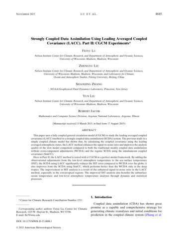
NOVEMBER 2015LU ET AL.4653FIG. 5. Zonal-mean RMSE of monthly SST from the SimCC experiment and the LACC experiments with different averaging lengths, normalized by the WCDA experiment.not be applicable to more general cases. Further studies are needed with different system configurations oreven other CGCMs.To apply the LACC method, the cross correlations between SST and time-averaged leading Ts are also estimated from the output of the control simulation (Fig. 3a)and the WCDA experiment (Fig. 3b). ‘‘Simultaneous’’indicates the same-day cross correlation as in Fig. 2, and‘‘AveX’’ means that cross correlation is calculated between SST and the average of X daily mean Ts from X 2 1days ago to the current one. Same as Fig. 2, all thetime-averaged leading Ts states are also spatial averages inorder to account for the coarser atmospheric resolutionand the covariance localization. The leading averagedcorrelations initially increase with the averaging length forall latitudes, and the increases are more noteworthy outside the tropics because of the higher correlations when Tsleads SST in Fig. 2. The correlations plateau when theaveraging length reaches 10 days in the deep tropics and20–30 days in the midlatitudes. As in Fig. 2, the correlations from the WCDA experiment are smaller than thosefrom the control simulation across all latitudes and averaging lengths. Together, Figs. 2 and 3 show that the simplecoupled model in Part I captures some important physicaland statistical features of the coupled ocean–atmospheresystem in a complex CGCM like FOAM, demonstratingthe potential application of LACC method to a SCDAsystem in a CGCM.Figure 4 shows the spatial distribution of two leadingaveraged cross correlations from the WCDA experiment,the simultaneous and the Ave7, along with the differencebetween the two distributions. In Fig. 4a, the simultaneouscorrelation is small except in the eastern tropical Pacific,which reflects the slow ENSO variability and its strongimpact on the atmosphere above. By averaging the 7-dayleading Ts (Fig. 4b), the cross correlation is significantlyenhanced across the displayed domain. The increasesfrom simultaneous to Ave7 (Fig. 4c) are the most notablein the extratropics, while most tropical locations showmuch less increase. We should note that, on purpose, allthe correlations shown in Figs. 2, 3, and 4 are estimationsof the coupled correlations from the control simulation orthe WCDA experiment instead of the exact correlationscalculated during the cross update of the SCDA experiment. The ability to estimate these correlations from thecontrol or WCDA provides valuable information abouthow much the SCDA and LACC method would improvethe analysis before their implementation.b. LACC experimentsNow we apply the LACC method to the cross updatethat assimilates the observations of low-level atmosphere temperature into the SST. We will show that,although the direct SCDA using simultaneous crosscovariance (SimCC) fails to improve upon the WCDA,the SCDA with the LACC method can indeed improveupon the WCDA significantly. Figure 5 shows a summary of the performance of the SimCC and the LACCmethod with different averaging lengths, normalizedby the WCDA. Following the notation of Fig. 3,‘‘AveX’’ means that cross update is done every X dayswith the X-day-averaged leading Ts . The SimCC methodperforms poorly across all latitudes except for the deeptropics between

(LACC) method for the SCDA. In a typical extratropical coupled ocean-atmosphere system, the cross correlation shows a strong asymmetry with the maximum correlation occurring when the atmosphere leads the ocean by about the decorrelation time of the atmosphere (Hasselmann 1976; Barsugli and Battisti 1998). The LACC method