Transcription
Discovering Partial Least Squareswith JMP Ian Cox and Marie Gaudard
ContentsPreface . xiA Word to the Practitioner. xiThe Organization of the Book . xiRequired Software . xiiAccessing the Supplementary Content . xiiChapter 1 Introducing Partial Least Squares. 1Modeling in General . 1Partial Least Squares in Today’s World . 2Transforming, and Centering and Scaling Data . 3An Example of a PLS Analysis . 4The Data and the Goal. 4The Analysis . 5Testing the Model . 9Chapter 2 A Review of Multiple Linear Regression . 11The Cars Example . 11Estimating the Coefficients . 15Underfitting and Overfitting: A Simulation . 16The Effect of Correlation among Predictors: A Simulation . 18Chapter 3 Principal Components Analysis: A Brief Visit . 25Principal Components Analysis . 25Centering and Scaling: An Example . 25Cox, Ian and Marie Gaudard. Discovering Partial Least Squares with JMP . Copyright 2013, SAS Institute, Inc., Cary, North Carolina,USA. ALL RIGHTS RESERVED.
viThe Importance of Exploratory Data Analysis in Multivariate Studies . 31Dimensionality Reduction via PCA . 34Chapter 4 A Deeper Understanding of PLS . 37Centering and Scaling in PLS . 37PLS as a Multivariate Technique . 38Why Use PLS?. 39How Does PLS Work? . 45PLS versus PCA . 49PLS Scores and Loadings . 50Some Technical Background . 50An Example Exploring Prediction . 59One-Factor NIPALS Model . 60Two-Factor NIPALS Model . 63Variable Selection . 64SIMPLS Fits . 64Choosing the Number of Factors . 65Cross Validation . 65Types of Cross Validation . 66A Simulation of K-Fold Cross Validation . 69Validation in the PLS Platform . 69The NIPALS and SIMPLS Algorithms . 71Useful Things to Remember About PLS . 72Chapter 5 Predicting Biological Activity . 75Background . 75The Data . 76Data Table Description. 76Initial Data Visualization . 77A First PLS Model . 79Our Plan . 79Performing the Analysis . 79The Partial Least Squares Report . 81The SIMPLS Fit Report . 82Other Options . 83A Pruned PLS Model . 93Cox, Ian and Marie Gaudard. Discovering Partial Least Squares with JMP . Copyright 2013, SAS Institute, Inc., Cary, North Carolina,USA. ALL RIGHTS RESERVED.
viiModel Fit . 93Diagnostics . 95Performance on Data from Second Study . 96Comparing Predicted Values for the Second Study to Actual Values . 96Comparing Residuals for Both Studies . 99Obtaining Additional Insight . 101Conclusion . 104Chapter 6 Predicting the Octane Rating of Gasoline . 105Background . 105The Data . 106Data Table Description. 106Creating a Test Set Indicator Column . 107Viewing the Data . 108Octane and the Test Set . 108Creating a Stacked Data Table . 109Constructing Plots of the Individual Spectra . 111Individual Spectra . 112Combined Spectra . 113A First PLS Model . 116Excluding the Test Set . 116Fitting the Model . 117The Initial Report . 118A Second PLS Model . 120Fitting the Model . 120High-Level Overview . 120Diagnostics . 121Score Scatterplot Matrices . 125Loading Plots . 127VIPs . 129Model Assessment Using Test Set . 133A Pruned Model . 136Chapter 7 Equation Chapter 1 Section 1Water Quality in the SavannahRiver Basin . 139Background . 140The Data . 141Cox, Ian and Marie Gaudard. Discovering Partial Least Squares with JMP . Copyright 2013, SAS Institute, Inc., Cary, North Carolina,USA. ALL RIGHTS RESERVED.
viiiData Table Description. 141Initial Data Visualization . 144Missing Response Values . 145Impute Missing Data . 146Distributions . 147Transforming AGPT . 148Differences by Ecoregion . 150Conclusions from Visual Analysis and Implications . 155A First PLS Model for the Savannah River Basin . 155Our Plan . 155Performing the Analysis . 156The Partial Least Squares Report . 159The NIPALS Fit Report . 159Defining a Pruned Model . 163A Pruned PLS Model for the Savannah River Basin . 166Model Fit . 166Diagnostics . 168Saving the Prediction Formulas . 169Comparing Actual Values to Predicted Values for the Test Set . 170A First PLS Model for the Blue Ridge Ecoregion . 173Making the Subset . 173Reviewing the Data . 174Performing the Analysis . 175The NIPALS Fit Report . 176A Pruned PLS Model for the Blue Ridge Ecoregion . 178Model Fit . 178Comparing Actual Values to Predicted Values for the Test Set . 179Conclusion . 181Chapter 8 Baking Bread That People Like . 183Background . 183The Data . 184Data Table Description. 184Missing Data Check . 186The First Stage Model . 187Visual Exploration of Overall Liking and Consumer Xs . 187Cox, Ian and Marie Gaudard. Discovering Partial Least Squares with JMP . Copyright 2013, SAS Institute, Inc., Cary, North Carolina,USA. ALL RIGHTS RESERVED.
ixThe Plan for the First Stage Model . 189Stage One PLS Model . 190Stage One Pruned PLS Model . 195Stage One MLR Model . 197Comparing the Stage One Models . 200Visual Exploration of Ys and Xs . 202Stage Two PLS Model . 207Stage Two MLR Model . 212The Combined Model for Overall Liking . 215Constructing the Prediction Formula . 215Viewing the Profiler . 218Conclusion . 219Appendix 1: Technical Details. 221Ground Rules . 222The Singular Value Decomposition of a Matrix . 222Definition. 222Relationship to Spectral Decomposition . 223Other Useful Facts . 223Principal Components Regression . 223The Idea behind PLS Algorithms . 224NIPALS . 225The NIPALS Algorithm. 225Computational Results . 228Properties of the NIPALS Algorithm . 231SIMPLS . 237Optimization Criterion . 237Implications for the Algorithm . 237The SIMPLS Algorithm . 238More on VIPs. 244The Standardize X Option . 246Determining the Number of Factors. 246Cross Validation: How JMP Does It . 246Appendix 2: Simulation Studies . 249Introduction . 249The Bias-Variance Tradeoff in PLS . 250Cox, Ian and Marie Gaudard. Discovering Partial Least Squares with JMP . Copyright 2013, SAS Institute, Inc., Cary, North Carolina,USA. ALL RIGHTS RESERVED.
xIntroduction . 250Two Simple Examples . 250Motivation . 254The Simulation Study . 255Results and Discussion . 257Conclusion . 261Using PLS for Variable Selection . 263Introduction . 263Structure of the Study . 264The Simulation . 267Computation of Result Measures . 268Results . 270Conclusion . 280References . 281Index . 285Cox, Ian and Marie Gaudard. Discovering Partial Least Squares with JMP . Copyright 2013, SAS Institute, Inc., Cary, North Carolina,USA. ALL RIGHTS RESERVED.
5Predicting Biological ActivityBackground . 75The Data . 76Data Table Description. 76Initial Data Visualization . 77A First PLS Model . 79Our Plan . 79Performing the Analysis . 79The Partial Least Squares Report . 81The SIMPLS Fit Report . 82Other Options . 83A Pruned PLS Model . 93Model Fit . 93Diagnostics . 95Performance on Data from Second Study. 96Comparing Predicted Values for the Second Study to Actual Values. 96Comparing Residuals for Both Studies . 99Obtaining Additional Insight . 101Conclusion . 104BackgroundThe example in this chapter comes from the field of drug discovery. New drugs aredeveloped from chemicals that are biologically active. Because testing a compound forbiological activity is expensive, chemists attempt to predict biological activity from othercheaper chemical measurements. In fact, computational chemistry makes it possible toCox, Ian and Marie Gaudard. Discovering Partial Least Squares with JMP . Copyright 2013, SAS Institute, Inc., Cary, North Carolina,USA. ALL RIGHTS RESERVED.
76 Discovering Partial Least Squares with JMPcalculate likely values for certain chemical properties without even making thecompound.In this example, you study the relationship between the size, hydrophobicity, andpolarity of key chemical groups at various sites on the molecule, and the activity of thecompound. The latter is represented by the logarithm of the relative Bradykininpotentiating activity. We develop a model based on a set of data from one study and thenwe apply the model to a separate data set from another study. For the first study, youlearn that PLS is a useful tool for finding a few underlying factors that account for mostof the variation in the response. However, you will also see that the model developedbased on the first study’s data set does not extend well to the data set from the secondstudy.The DataData Table DescriptionOpen the data table Penta.jmp, partially shown in Figure 5.1, by clicking on the link inthe master journal. This table contains 30 rows of observations.The column obsnam contains an identification code. Each record in Penta.jmp representsa peptide chain of five amino acids. Each amino acid name is coded using a single letterand each chain is represented by five letters, as shown in the column obsnam. The aminoacid coding is described in Table 1 of Hellberg et al. (1986).The response of interest is rai, a relative measure of Bradykinin potentiating activity. (SeeTable 1 in both Ufkes et al. 1978 and Ufkes et al. 1982). However, rai is highly skewed,and so log rai, the base 10 logarithm of rai, is used as the response of interest in theanalysis. Note that log rai is given by a formula; click the sign next to log rai in theColumns panel to view the formula.The first column in the data table, Study, indicates the study of origin for the given row.The first 15 observations in the table were studied in Ufkes et al. (1978) and the last 15 inUfkes et al. (1982).Cox, Ian and Marie Gaudard. Discovering Partial Least Squares with JMP . Copyright 2013, SAS Institute, Inc., Cary, North Carolina,USA. ALL RIGHTS RESERVED.
Chapter 5 Predicting Biological Activity 77Figure 5.1: Partial View of Penta.jmpThe data used in this example and a discussion can be found in SAS documentation(SAS/STAT 9.3 User’s Guide, “The PLS Procedure”). To facilitate comparisons with SASoutput, our analysis broadly follows the steps used in the PROC PLS example (Example69.1). Further background on the data can be found in Ufkes et al. (1978) and Ufkes et al.(1982), Sjostrom and Wold (1985), and Hellberg et al. (1986).Initial Data VisualizationLet’s start by visualizing the data. Run the first saved script, Distribution of rai andlog rai. The plot for rai in Figure 5.2 shows that rai is highly skewed, with some largeoutlying values.Cox, Ian and Marie Gaudard. Discovering Partial Least Squares with JMP . Copyright 2013, SAS Institute, Inc., Cary, North Carolina,USA. ALL RIGHTS RESERVED.
78 Discovering Partial Least Squares with JMPFigure 5.2: Distribution Reports for rai and log raiAlthough PLS does not rely on distributional assumptions of normality, it is still goodpractice to look at the univariate distributions of the variables and assess whether one ofthe familiar transformations can make the
Open the data table Penta.jmp, partially shown in Figure 5.1, by clicking on the link in the master journal. This table contains 30 rows of observations. The column obsnam contains an identification code. Each recordin Penta.jmp represents a peptide chain of five amino acids. Each amino acid name is coded using a single letter