Transcription
Crash Course on Basic StatisticsMarina Wahl, marina.w4hl@gmail.comUniversity of New York at Stony BrookNovember 6, 2013
2
Contents1 Basic Probability1.1 Basic Definitions . . . . . . . . . . . . . . . . . . . . . . . . . . . . . . . . . . . . . . . . . . .1.2 Probability of Events . . . . . . . . . . . . . . . . . . . . . . . . . . . . . . . . . . . . . . . . .1.3 Bayes’ Theorem . . . . . . . . . . . . . . . . . . . . . . . . . . . . . . . . . . . . . . . . . . . .55662 Basic Definitions2.1 Types of Data . . . . . . .2.2 Errors . . . . . . . . . . .2.3 Reliability . . . . . . . . .2.4 Validity . . . . . . . . . .2.5 Probability Distributions .2.6 Population and Samples .2.7 Bias . . . . . . . . . . . .2.8 Questions on Samples . .2.9 Central Tendency . . . . .7777778899.3 The Normal Distribution114 The Binomial Distribution135 Confidence Intervals156 Hypothesis Testing177 The t-Test198 Regression239 Logistic Regression2510 Other Topics2711 Some Related Questions293
4CONTENTS
Chapter 1Basic Probability1.1Basic Definitions? The probability of an event is always between0 and 1.Trials? The probability of an event and its complementis always 1.? Probability is concerned with the outcome of trials.Several Events? Trials are also called experiments or observations (multiple trials).? The union of several simple events creates acompound event that occurs if one or moreof the events occur.? Trials refers to an event whose outcome is unknown.? The intersection of two or more simple eventscreates a compound event that occurs only ifall the simple events occurs.Sample Space (S)? Set of all possible elementary outcomes ofa trial.? If events cannot occur together, they are mutually exclusive.? If the trial consists of flipping a coin twice, thesample space is S (h, h), (h, t), (t, h), (t, t).? If two trials are independent, the outcome ofone trial does not influence the outcome of another.? The probability of the sample space is always1.PermutationsEvents (E)? Permutations are all the possible ways elements in a set can be arranged, where the orderis important.? An event is the specification of the outcome ofa trial.? An event can consist of a single outcome or aset of outcomes.? The number of permutations of subsets of size kdrawn from a set of size n is given by:? The complement of an event is everything inthe sample space that is not that event (not Eor E).nP k 5n!(n k)!
6CHAPTER 1. BASIC PROBABILITYCombinations– There are true, fixed parameters in a model(though they may be unknown at times).? Combinations are similar to permutations withthe difference that the order of elements isnot significant.– Data contain random errors which have acertain probability distribution (Gaussianfor example).? The number of combinations of subsets of size kdrawn from a set of size n is given by:nP k 1.2n!k!(n k)!– Mathematical routines analyse the probability of getting certain data, given a particular model.? Bayesian:Probability of Events? If two events are independents, P (E F ) P (E). The probability of both E and F occurring is:P (E F ) P (E) P (F )? If two events are mutually exclusive, the probability of either E or F :P (E F ) P (E) P (F )? If the events are not mutually exclusive (youneed to correct the ‘overlap’):P (E F ) P (E) P (F ) P (E F ),whereP (E F ) P (E) P (F E)1.3Bayes’ TheoremBayes’ theorem for any two events:P (A B) P (A B)P (B A)P (A) P (B)P (B A)P (A) P (B A)P ( A)? Frequentist:– There are no true model parameters. Instead all parameters are treated as randomvariables with probability distributions.– Random errors in data have no probabilitydistribution, but rather the model parameters are random with their own distributions.– Mathematical routines analyze probabilityof a model, given some data. The statistician makes a guess (prior distribution) andthen updates that guess with the data.
Chapter 2Basic Definitions2.1Types of Data? Internal consistency reliability: how wellthe items that make up instrument (a test) reflect the same construct.There two types of measurements:? Quantitative: Discrete data have finite values. Continuous data have an infinite numberof steps.2.4Validity? Categorical (nominal): the possible responses How well a test or rating scale measures whatconsist of a set of categories rather than numbers is supposed to measure:that measure an amount of something on a con? Content validity: how well the process of meatinuous scale.surement reflects the important content of thedomain of interests.2.2Errors? Concurrent validity: how well inferencesdrawn from a measurement can be used to predict some other behaviour that is measured atapproximately same time.? Random error: due to chance, with no particular pattern and it is assumed to cancel itself outover repeated measurements.? Systematic errors: has an observable pattern,and it is not due to chance, so its causes can beoften identified.2.3? Predictive validity: the ability to draw inferences about some event in the future.2.5ReliabilityProbability Distributions? Statistical inference relies on making assumptions about the way data is distributed, transforming data to make it fit some known distribution better.How consistent or repeatable measurements are:? Multiple-occasions reliability (test-retest,temporal): how similarly a test perform overrepeated administration.? A theoretical probability distribution is defined by a formula that specifies what values canbe taken by data points within the distributionand how common each value (or range) will be.? Multiple-forms reliability (parallel-forms):how similarly different versions of a test performin measuring the same entity.7
8CHAPTER 2. BASIC DEFINITIONS2.6Population and Samples– Calculate n by dividing the size of the population by the number of subjects you wantin the sample.? We rarely have access to the entire population ofusers. Instead we rely on a subset of the population to use as a proxy for the population.– Useful when the population accrues overtime and there is no predetermined listof population members.? Sample statistics estimate unknown population parameters.– One caution: making sure data is not cyclic.? Ideally you should select your sample randomly from the parent population, but in practice this can be very difficult due to:? Stratified sample: the population of interestis divided into non overlapping groups or stratabased on common characteristics.– issues establishing a truly random selectionscheme,? Cluster sample: population is sampled by using pre-existing groups. It can be combined withthe technique of sampling proportional to size.– problems getting the selected users to participate.? Representativeness is more important than randomness.Nonprobability Sampling? Subject to sampling bias. Conclusions are of limited usefulness in generalizing to a larger population:2.7Bias? Sample needs to be a good representation of thestudy population.? If the sample is biased, it is not representativeof the study population, conclusions draw fromthe study sample might not apply to the studypopulation.– Convenience samples: collect information in the early stages of a study.? A statistic used to estimate a parameter is unbiased if the expected value of its sampling distribution is equal to the value of the parameterbeing estimated.– Quota sampling: the data collector isinstructed to get response from a certainnumber of subjects within classifications.? Bias is a source of systematic error and enterstudies in two primary ways:– Volunteer samples.Probability Sampling? Every member of the population has a knowprobability to be selected for the sample.? The simplest type is a simple random sampling (SRS).? Systematic sampling: need a list of your population and you decide the size of the sample andthen compute the number n, which dictates howyou will select the sample:– During the selection and retention ofthe subjects of study.– In the way information is collectedabout the subjects.Sample Selection Bias? Selection bias: if some potential subjects aremore likely than others to be selected for thestudy sample. The sample is selected in a waythat systematically excludes part of the population.
2.9. CENTRAL TENDENCY? Volunteer bias: the fact that people who volunteer to be in the studies are usually not representative of the population as a whole.? Nonresponse bias: the other side of volunteerbias. Just as people who volunteer to take partin a study are likely to differ systematically fromthose who do not, so people who decline to participate in a study when invited to do so verylikely differ from those who consent to participate.? Informative censoring: can create bias in anylongitudinal study (a study in which subjects arefollowed over a period of time). Losing subjectsduring a long-term study is common, but thereal problem comes when subjects do not dropout at random, but for reasons related to thestudy’s purpose.Information Bias? Interviewer bias: when bias is introduced intro the data collected because of the attitudes orbehaviour of the interviewer.? Recall bias: the fact that people with a life experience such as suffering from a serious diseaseor injury are more likely to remember events thatthey believe are related to that experience.? Detection bias: the fact that certain characteristics may be more likely to be detected orreported in some people than in others.? Social desirability bias: caused by people’sdesire to present themselves in a favorable light.9Bias? Response Bias: how were the questions wordedand the response collected? Concious Bias: are arguments presented in a disinterested, objective fashion? Missing data and refusals: how is missing datatreated in the analysis? How is attrition (loss ofsubjects after a study begins) handled?Sample Size? Were the sample sizes selected large enough fora null hypothesis to be rejected? Were the sample sizes so large that almost anynull hypothesis would be rejected? Was the sample size selected on the basis of apower calculation?2.9Central TendencyMean? Good if data set that is roughly symmetrical:nµ 1Xxi .n i 1? Outliers: data error or they belong to otherpopulation.Median2.8Questions on SamplesRepresentative Sampling? How was the sample selected? Was it truly randomly selected? Were there any biases in the selection process? Middle value when the values are ranked in ascending or descending order.? When data is not symmetrical, mean can beheavily influenced by outliers, and median provides a better idea o most typical value.? For odd samples, the median is the central value(n 1)/2th. For even samples, it’s the averageof the two central values, [n/2 (n 1)/2]/2th.
10CHAPTER 2. BASIC DEFINITIONS? In a small sample of data (less than 25 or so),the sample median tends to do a poor job ofestimating the population median.? For task-time data the geometric meantends to provide a better estimate of the population’s middle value than the sample median.Mode? The most frequently occurring value.? Is useful in describing ordinal or categorical data.Dispersion? Range: simplest measure of dispersion, whichis the difference between the highest and lowestvalues.? Interquartile range: less influenced by extreme values.? Variance:– The most common way to do measure dispersion for continuous data.– Provides an estimate of the average difference of each value from the mean.– For a population:nσ2 1X(xi µ)2n i 1– For a sample:ns2 1 X(xi x̄)2n 1 i 1? Standard deviation:– For a population: σ σ2 ,– For a sample: s s2 .
Chapter 3The Normal Distributionmal distribution regardless of what the parentpopulation’s distribution (usually 30 or larger).? The mean of this distribution of samplemeans will also be equal to the mean of theparent population. If X1 , X2 , ., Xn all havemean µ Pand variance σ 2 , sampling distributionof X̄ nXi :Figure 3.1: (left) All normal distributions have thesame shape but differ to their µ and σ: they areshifted by µ and stretched by σ. (right) Percent ofdata failing into specified ranges of the normal distribution.E(X̄) µ, V ar(X̄,using the central limit theorem, for large n, X̄ 2N (µ, σn ).? If we are interested on p, a proportion or theprobability of an event with 2 outcomes. We usethe estimator p̂, proportion of times we see theevent in the data. The sampling distribution ofp̂ (unbiased estimator ofqp) has expected value p? All normal distributions are symmetric,unimodal (a single most common value), andhave a continuous range from negative infinityto positive infinity.and standard deviation p(1 p). By the centralnlimit theorem, for large n the sampling distribution is p̂ N (p, p(1 p)).n? The total area under the curve adds up to 1, or100%.? Empirical rule: For the population that follows a normal distribution, almost all the valueswill fall within three standard deviations aboveand bellow the mean (99.7%). Two standard deviations are about 95%. One standard deviationis 68%.σ2),nThe Z-Statistic? A z-score is the distance of a data point from themean, expressed in units of standard deviation.The z-score for a value from a population is:Z The Central Limit Theorem? As the sample size approaches infinity, the distribution of sample means will follow a nor11x µσ? Conversion to z-scores place distinct populationson the same metric.
12CHAPTER 3. THE NORMAL DISTRIBUTION? We are interested in the probability of a particular sample mean. We can use the normaldistribution even if we do not know the distribution of the population from which the samplewas drawn, by calculating the z-statistics:Z x̄ µ σn.? The standard error of the mean σn is thestandard deviation of the sampling distributionof the sample mean:– It describes the mean of multiple members of a population.– It is always smaller than the standard deviation.– The larger our sample size is, the smaller isthe standard error and less we would expectour sample mean to differ from the population mean.? If we know the mean but not the standard deviation, we can calculate the t-statistic instead(following sessions).
Chapter 4The Binomial Distribution? An example of discrete distribution? Events in a binomial distribution are generated by a Bernoulli process. A single trialwithin a Bernoulli process is called a Bernoullitrial.? Data meets four requirements:– The outcome of each trial is one of two mutually exclusive outcomes.– Each trial is independent.– The probability of success, p, is constant forevery trial.– There is a fixed number of trials, denotedas n.? The probability of a particular number of successes on a a particular number of trials is: n kP (X k) p (1 p)n kkwhere nn! nCk kk!(n k)!? If both np and n(1 p) are grater than 5, thebinomial distribution can be approximated bythe normal distribution.13
14CHAPTER 4. THE BINOMIAL DISTRIBUTION
Chapter 5Confidence IntervalsPoint Estimate? Point estimate is a single statistic, such as themean, to describe a sample.? If we drew a different sample, the mean calculated from that sample would probably be different.? The confidence is in the method, not in any interval.? Any value inside the interval could be said to bea plausible value.? CI are twice the margin of error and provideboth a measure of location and precision.? Interval estimates state how much a point estimate is likely to vary by chance.? One common interval estimate is the confidence level, calculated as (1 α). where αis the significance.Confidence Interval? The confidence interval is the range of valuesthat we believe will have a specified chance ofcontaining the unknown population parameter.? The confidence interval is a range of valuesaround the mean for which if we drew an infinite number of samples of the same size fromthe same population, x% of the time the truepopulation mean would be included in the confidence interval calculated from the samples. Itgives us the information about the precision of apoint estimate such as the sample mean.? CI will tell you the most likely range of the unknown population mean or proportion.15? Three things affect the width of a confidence interval:– Confidence Level: usually 95%.– Variability: if there is more variation ina population, each sample taken will fluctuate more and wider the confidence interval. The variability of the population is estimated using the standard deviation fromthe sample.– Sample size: without lowering the confidence level, the sample size can control thewidth of a confidence interval, having aninverse square root relationship to it.CI for Completion Rate (Binary Data)? Completion rate is one of the most fundamental usability metrics, defining whether auser can complete a task, usually as a binaryresponse.
16CHAPTER 5. CONFIDENCE INTERVALS? The first method to estimate binary success ratesis given by the Wald interval:rp̂(1 p̂)αp̂ z(1 2 ),nwhere p̂ is the sample proportion, n is the samplesize, z(1 α2 ) is the critical value from the normaldistribution for the level of confidence.? Very inaccurate for small sample sizes (less than100) or for proportions close to 0 or 1.? For 95% (z 1.96) confidence intervals, we canadd two successes and two failures to the observed number of successes and failures:2p̂adj ? We also want our sample mean to be unbiased,where any sample mean is just as likely to overestimate or underestimate the population mean.The median does not share this property: atsmall samples, the sample median of completion times tends to consistently overestimatedthe population median.? For small-sample task-time data the geometricmean estimates the population median betterthan the sample median. As the sample sizesget larger (above 25) the median tends to be thebest estimate of the middle value. We can usebinomial distribution to estimate the confidenceintervals: the following formula constructs a confidence interval around any percentile. The median (0.5) would be the most common:2x 1.96x z2x 22 ,2n zn 1.962n 4(5.0.1)where x is the number that successfully completed the task and n the number who attemptedthe task (sample size).CI for Task-time Data? Measuring time on task is a good way to assess task performance and tend to be positivelyskewed (a non-symmetrical distribution, so themean is not a good measure of the center of thedistribution).? In this case, the median is a better measure of thecenter. However, there is two major drawbacksto the median: variability and bias.? The median does not use all the informationavailable in sample, consequently, the medians ofsamples from a continuous distribution are morevariable than their means.? The increased variability of the median relativeto the mean is amplified when the sample sizesare small.np z(1 α2 )pnp(1 p),where n is the sample size, ppis the percentileexpressed as a proportion, and np(1 p) is thestandard error. The confidence interval aroundthe median is given by the values taken by theth integer values in this formula (in the ordereddata set).
Chapter 6Hypothesis Testing? H0 is called the null hypothesis and H1 is thealternative hypothesis. They are mutually exclusive and exhaustive. A null hypothesis cannotnever be proven to be true, it can only be shownto be plausible.? The alternative hypothesis can be single-tailed:it must achieve some value to reject the null hypothesis,strong enough to support rejection of the nullhypothesis.? Expresses the probability that extreme resultsobtained in an analysis of sample data are dueto chance.? A low p-value (for example, less than 0.05)means that the null hypothesis is unlikely to betrue.H0 : µ1 µ2 , H1 : µ1 µ2 ,or can be two-tailed: it must be different fromcertain value to reject the null hypothesis,H0 : µ1 µ2 , H1 : µ1 6 µ2 .? With null hypothesis testing, all it takes is sufficient evidence (instead of definitive proof) thatwe can see as at least some difference. The size ofthe difference is given by the confidence intervalaround the difference.? A small p-value might occur:? Statistically significant is the probability thatis not due to chance.? If we fail to reject the null hypothesis (find significance), this does not mean that the null hypothesis is true, only that our study did not findsufficient evidence to reject it.? Tests are not reliable if the statement of thehypothesis are suggested by the data: datasnooping.– by chance– because of problems related to data collection– because of violations of the conditions necessary for testing procedure– because H0 is true? if multiple tests are carried out, some are likelyto be significant by chance alone! For σ 0.05,we expect that significant results will be 5% ofthe time.p-value? We choose the probability level or p-value thatdefines when sample results will be considered17? Be suspicious when you see a few significant results when many tests have been carried out orsignificant results on a few subgroups of the data.
18CHAPTER 6. HYPOTHESIS TESTINGErrors in Statistics? If we wrongly say that there is a difference,we have a Type I error. If we wrongly saythere is no difference, it is called Type IIerror.? Setting α 0.05 means that we accept a 5%probability of Type I error, i.e. we have a 5%chance of rejecting the null hypothesis when weshould fail to reject it.? Levels of acceptability for Type II errors are usually β 0.1, meaning that it has 10% probability of a Type II error, or 10% chance that thenull hypothesis will be false but will fail to berejected in the study.? The reciprocal of Type II error is power, definedas 1 β and is the probability of rejecting thenull hypothesis when you should reject it.? Power of a test:– The significance level α of a test shows howthe testing methods performs if repeatedsampling.– If H0 is true and α 0.01, and you carryout a test repetitively, with different samples of the same size, you reject the H0(type I) 1 per cent of the time!– Choosing α to be very small means that youreject H0 even if the true value is differentform H0 .? The following four main factors affect power:– α level (higher probability of Type I errorincreases power).– Difference in outcome between populations(greater difference increases power).– Variability (reduced variability increasespower).– Sample size (larger sample size increasespower).? How to have a higher power:– The power is higher the further the alternative values away from H0 .– Higher significance level α gives higherpower.– Less variability gives higher power.– The larger the samples size, the greater isthe power.
Chapter 7The t-Testt-Distribution? The t-distribution adjusts for how good ourestimative is by making the intervals wider asthe sample sizes get smaller. It converges to thenormal confidence intervals when the sample sizeincreases (more than 30).? Two main reasons for using the t-distributionto test differences in means: when working withsmall samples from a population that is approximately normal, and when we do not know thestandard deviation of a population and need touse the standard deviation of the sample as awhere x̄ is the sample mean, n is the sample size, ssubstitute for the population deviation.is the sample standard deviation, t(1 α2 ) is the crit? t-distributions are continuous and symmetrical, ical value from the t-distribution for n 1 degreesand a bit fatter in the tails.of freedom and the specified level of confidence, we? Unlike the normal distribution, the shape of the need:t distribution depends on the degrees of freedomfor a sample.? At smaller sample sizes, sample means fluctuatemore around the population mean. For example, instead of 95% of values failing with 1.96standard deviations of the mean, at a sample sizeof 15, they fall within 2.14 standard deviations.1. the mean and standard deviation of the mean,2. the standard error,3. the sample size,4. the critical value from the t-distribution for thedesired confidence level.The standard error is the estimate of how much theConfidence Interval for t-Distributions average sample means will fluctuate around the truepopulation mean:To construct the interval,sx̄ t(1 α2 ) ,nsse .n19
20CHAPTER 7. THE T-TESTThe t-critical value is simply:t x̄ µ sn,hypothesis is that there is no significant difference between the mean population from which your samplewas drawn and the mean of the know population.The standard deviation of the sample is:sPwhere we need α (level of significance, usually 0.05,n2i 1 (xi x̄)one minus the confidence level) and the degrees ofs n 1freedom. The degrees of freedom (df) for this type ofconfidence interval is the sample size minus 1.The degrees of freedom for the one sample t-test isFor example, a sample size of 12 has the expectan 1.tion that 95% of sample means will fall within 2.2standard deviations of the population mean. We canalso express this as the margin of error:CI for the One-Sample t-TestsThe formula to compute a two-tailed confidence inme 2.2 ,nterval for the mean for the one-sample t-test:and the confidence interval is given as twice the mg.t-testAssumptions of t-tests:? The samples are unrelated/independent, otherwise the paired t-test should be used. You cantest for linear independence. s CI1 α x̄ tα/2,df nIf you want to calculate a one-sided CI, change the sign to either plus or minus and use the uppercritical value and α rather than α/2.2-Sample t-Test (Independent Sam-? t-tests assume that the underlying population ples)variances of the two groups are equal (variancesare pooled), so you should test for homogeneity. The t-test for independent samples determineswhether the means of the populations from which the? Normality of the distributions of both variables samples were drawn are the same. The subjects inare also assumed (unless the samples sizes are the two samples are assumed to be unrelated and inlarge enough to apply the central limit theorem). dependently selected from their populations. We assume that the populations are approximately a nor? Both samples are representative of their parent mal distribution (or sample large enough to invokepopulations.the central limit theorem) and that the populations? t-tests are robust even for small sample sizes, ex- have approximately equal variance:cept when there is an extreme skew distributionor outliers.1-Sample t-TestOne way t-test is used is to compare the mean of asample to a population with a known mean. The nullt (x̄1 x̄2 ) (µ1 µ2 )r , 112sp n1 n2where the pooled variance iss2p (n1 1)s21 (n2 1)s22.n1 n2 2
21Comparing SamplesCI for the Independent Samples t-TestCI1 α r 11 s2p (x̄1 x̄2 ) tα/2,df n1n2 !The concept of the number of standard errors that thesample means differ from population means applies toboth confidence intervals and significance tests.The two-sample t-test is found by weighting theaverage of the variances:Repeated Measures t-Testx̂1 x̂2t r 2 ,s1Also know as related samples t-test or the depens2dent samples t-tests, the samples are not indepenn1 n22dent. The measurements are considered as pairs sothe two samples must be of the same size. The for- where x̂1 and x̂2 are the means from sample 1 andmula is based on the difference scores as calculated 2, s1 and s2 the standard deviations from sample 1from each pairs of samples:and 2, and n1 and n2 the sample sizes. The degreeof freedom for t-values is approximately 2 less thed (µ1 µ2 )smaller of the two sample sizes. A p-value is just a,t sd percentile rank or point in the t-distribution.nThe null hypothesis for an independent sampleswhere d is the mean of the different scores and n the t-test is that the difference between the populationnumber of pairs. The degrees of freedom is still n 1. means is 0, in which case µ1 µ2 ) can be dropped.The null hypothesis for the repeated measures t- The degree of freedom is n1 n2 2, fewer than thetest is usually that the mean of the difference scores, number of cases when both samples are combined. is 0.d,CI for the Repeated Measures t-Test s dCI1 α d tα/2,df nTwo Measurements? H0 : µ µ0 , HA : µ 6 µ0? observations: n, x̄, s, d x̄ µ0 ? Reject H0 ifP ( X̄ µ0 d) αX̄ µ0d P ( p p)2s /ns2 /nd P ( tn 1 p)s2 /nBetween-subjects Comparison (Twosample t-test)When a different set of users is tested on each product, there is variation both between users and between designs. Any difference between the meansmust be tested to see whether it is greater thanthe variation between the different users. To determine whether there is a significant difference betweenmeans of independent samples of users, we use thetwo-sample t-test:x̂1 x̂2t q 2s1s22n1 n2The degrees of freedom for one-sample t-test is n 1. For a two-sample t-test, a simple formula is n1 1n2 2. However the correct formula is given byWelch-Satterthwaite procedure. It provides accurate
22CHAPTER 7. THE T-TESTresults even if the variances are unequal: df s21n1s21n1 2n1 1s22n2 2s22n2 2n2 1CI Around the DifferenceThere are several ways to report an effect size, butthe most compelling and easiest to understand is theconfidence interval. The following formula generatesa confidence interval around the difference scores tounderstand the likely range of the true difference between products:ss21s2 2.(x̂1 x̂2 ) tan1n2
Chapter 8RegressionLinear Regression? It calculates the equation that will produce theline that is as close as possible to all the datapoints considered together. This is describedas minimizing the square deviations, where thesquared deviations are the sum of the squareddeviations b
Basic Probability 1.1 Basic De nitions Trials? Probability is concerned with the outcome of tri-als.? Trials are also called experiments or observa-tions (multiple trials).? Trials refers to an event whose outcome is un-known. Sample Space (S)? Set of all possible elementary outcomes of a trial.? If the trial consists of ipping a coin twice, theFile Size: 652KB